Introduction to Fractals
A Bit of History
The word "Fractal" was coined in 1975 by Poland born, France educated, and naturalized American mathematician Benoit Mandelbrot(1924 - 2010 ) to describe shapes which are detailed at all scales.His last name means "almond bread" in German.
The word is a variant of "fractional",since a fractal is a type of fractional dimension found in many naturally occuring physical phenomena.
Its Latin root is "fractus",which is recognizable in the native English break, suggesting fragmented, broken and discontinuous.
As a result, the word "fractal" is now used not only for objects with fractional dimension, but also for those with the property of
repeating
self-similar shapes even when they do not have a characteristic of fractional dimesion.
The first mathematical fractal was discovered in 1861 by
Karl Weierstrass(1815 - 1897).
Weierstrass's function was ,although continuous,completely made of corners, and nowhere differentiable.
It was not possible to define the rate of change anywhere.
This was a shock to the scientists of the day, and it was named "pathological curve".
The Cantor Set,which is now named after the German mathematician
Georg Cantor(1845 - 1918), the student of Weierstrass, is one of the
first fractals
to be studied mathematically. It was the year 1883.
But this was actually discovered by Henry Smith(1826 - 1883),
a professor of geometry at Oxford , in 1875.
The Cantor set has no length, and in mathematical terms,it has "zero measure". But how about its dimension ?
Mathematicians began searching for a new way of defining dimension.
Around 1890, an Italian mathemtician
Giuseppe Peano(1858 - 1932) surprised the mathematical world by dicovering what was called
"space-filling curve". His curve was constructed in such a way that there was no point on the plane that its twisted curve would not include.
It means that a line, which is considered as one dimensional object, has one to one mapping to all the points on the plane, which is
two dimensional.
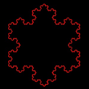
The other "pathological" curve was discovered in 1904 by a Swedish mathematician
Helge von Koch(1870 - 1924).
The finished curve,though contained in a finite area, has an infinite length ,
and has no smoothness, or tangent anywhere. It is now called Koch's snowflake or simply Koch curve.
What he did not know was that its property
of infinite length can be used as an ideal model for the shapes of the real world like coastlines,
and its dimension was later found being equal to (log 4)/(log 3) = 1.26... (it is fractal !!).
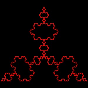
In 1916, the polish mathematician
Waclaw Sierpinski(1882 - 1969) introduced a fractal now called "Sierpinski Gasket" or
"Sierpinski Triangle".
Nowadays this fractal model figure can be seen in almost any books writtten about the topic of fractal.
During the late 19-th and early 20-th entury, another group of mathematicians began research on what is now called
"dynamical system", by iterating simple functions .
In 1979,British mathematician
Sir Arthur Cayley(1821 - 1895)
published a problem called "Newton-Fourier Imaginary Problem", in which
he proposed a new method of finding roots of algebraic equation using Newton's method in complex plane.
He wrote at the end of his one page article :
" The solution is easy and elegant in the case of a quadric equation , but the next succeeding case of the cubic equation appears to present considerable difficulty.", and
the paper on the cubic equation case has never been published by him. The reader will soon see the reason why it is so.
This paper motivated the French mathematician
Gaston Julia(1893 - 1978) and his compatriot and competitor
Pierre Fatou (1878 - 1929)
to do reseach in area of complex iteration.
In 1918,when Julia was only 25 years old, Julia published his 199 page masterpiece Mémoire sur l'itération des fonctions rationnelles,
(concerning the iteration of a rational function) . It received the Grand Prix de l'Académie des Sciences.
Although he was famous in the 1920s, his work was essentially forgotten until Benoit Mandelbrot brought it back to prominence in the 1970s through his fundamental computer experiments.
"Julia Set" and "Fatou set" are named after these two early reserchers to honor their great contributions.
In 1980 Benoit Madelbrot discovered "Mandelbrot Set" while he was experimenting with Julia Set using high speed computers.
Since then many mathematicians joined the bandwagon ,and many words like Chaos, Dynamical System, Fractal, etc has become the household names.
The readers will see only a little bit of this history in this section. There are a lot of good books and video tape available. They are lsted in the reference section
List of animations posted on this page.(Click the text to watch animation.)
Use browser's "Back" button to come back to this page.
Table of Contents
- 1. Self-Similarity
- 2. Space Filling curves
- 3. Fractal Tree, Dragon curves
- 4. Function Iteration and Newton's method
- 5. Julia Set
- 6. Mandelbrot Set
- 7. IFS(Iterated Funtion System)
1. Self-Similarity
1.1 Cantor Set
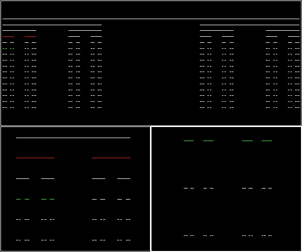
Take a line, remove the middle third,leaving two equal lines with length one third .Next , remove the middle thirds from these two lines, and continue the process an infinite number of times.
The resulting set of points is called the Cantor set, named after the German mathematician Georg Cantor(1845 - 1918).
This is one of the first fractals to be studied mathematically.
The picture below shows the first 15 steps.
One thing noticed immediately is that the zoomed pictures around "red" and "green" lines
are the scaled down copies of the total image.
This "self-similarity" is one of the characteristics of "FRACTAL".
******************************* Cantor.dwg *******************************
You can see the process in animation.
To create this drawing and animation:
Load fractal_mandelb.lsp (load "fractal_mandelb")
Then from command line, type Cantor
The picture below is another way of displaying Cantor set, called "Cantor comb".
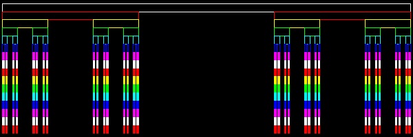
***************************** Cantor_comb.dwg *****************************
To create this drawing :
Load fractal_mandelb.lsp (load "fractal_mandelb")
Then from command line, type Cantor_comb
1.2 Koch Curves
Koch Curve
| Koch_base_0.dwg Initial stage  |
Koch_base_1.dwg First step 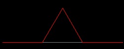 |
Koch_base_2.dwg Second step 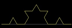 |
| Koch_base_3.dwg 3-rd step 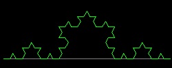 |
Koch_base_4.dwg 4-th step 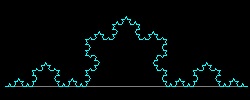 |
Koch_base_5.dwg 5-th step 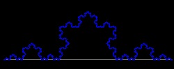 |
You can see the process in animation.
To create this drawing and animation:
Load snowflake.lsp (load "snowflake")
Then from command line, type Koch_base
Koch's Snowflake & anti-Snowflake
| snowflake_0.dwg Initial stage 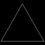 |
snowflake_1.dwg First step 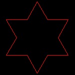 |
snowflake_2.dwg Second step 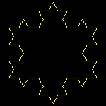 |
snowflake_3.dwg Third step 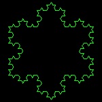 |
snowflake_4.dwg Fourth step 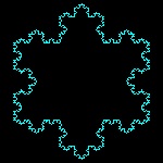 |
| snowflake_0.dwg Initial stage |
anti-snowflake_1.dwg First step 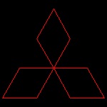 |
anti-snowflake_2.dwg Second step  |
anti-snowflake_3.dwg Third step  |
anti-snowflake_4.dwg Fourth step 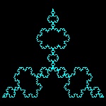 |
You can see the process in animation.
Snowflake animation
 |
Anti-snowflake animation
 |
To create this drawing and animation:
Load snowflake.lsp (load "snowflake")
Then from command line, type Koch_1 for Snowflake case
Then from command line, type Koch_2 for Anti-Snowflake case
1.3 Blancmange Curve
| blancmange_1.dwg Initial stage  |
blancmange_2.dwg Second step  |
blancmange_3.dwg Third step  |
blancmange_4.dwg 4-th step 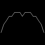 |
| blancmange_5.dwg 5-th stage 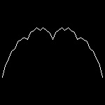 |
blancmange_6.dwg 6-th step 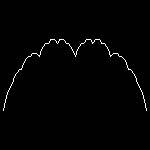 |
blancmange_7.dwg 7-th step 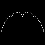 |
blancmange_8.dwg 8-th step 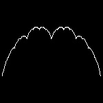 |
You can see the process in animation.
To create this drawing and animation:
Load blancmange.lsp (load "blancmange")
Then from command line, type blancmange
1.4 Sierpinski's Gasket
| gasket_1.dwg Initial stage 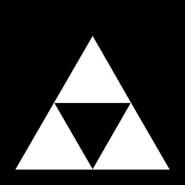 |
gasket_2.dwg Second step 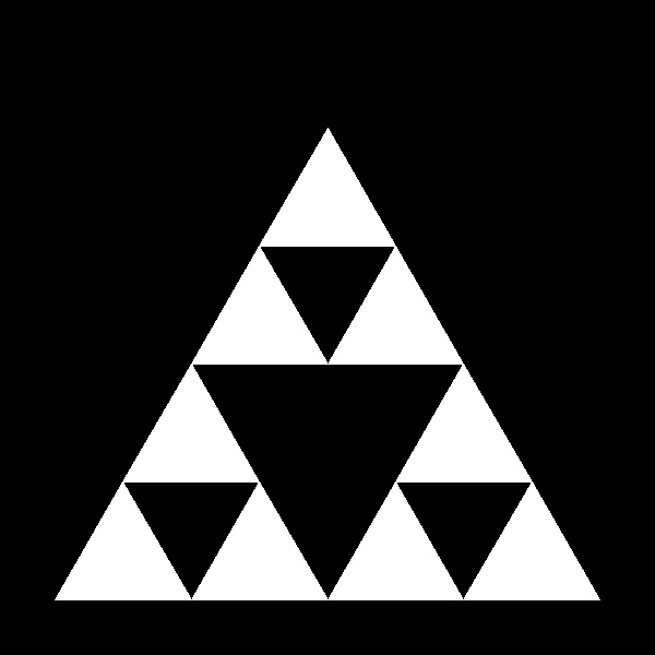 |
gasket_4.dwg 4-th step 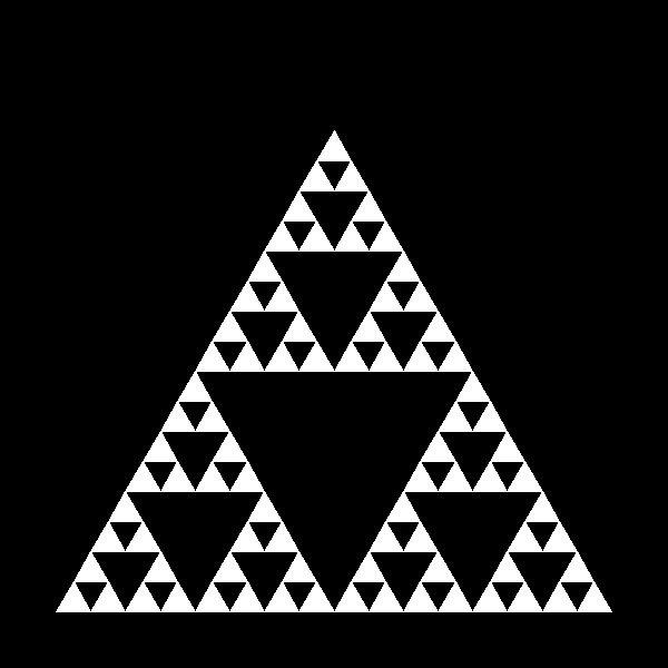 |
gasket_8.dwg 8-th step 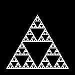 |
| maze_1.dwg Initial stage 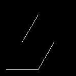 |
maze_2.dwg 2-nd step 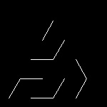 |
maze_4.dwg 4-th step 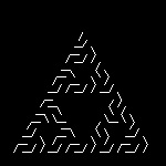 |
maze_8.dwg 8-th step 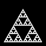 |
| arrowhead_1.dwg Initial stage 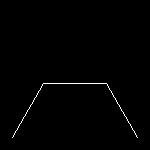 |
arrowheade_2.dwg Second step 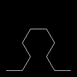 |
arrowhead_4.dwg 4-th step 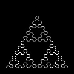 |
arrowhead_8.dwg 8-th step 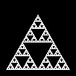 |
Sierpinski Gasket:
You can see the process in animation.
To create this drawing and animation:
Load sierpinski_gaske.lsp (load "sierpinski_gaske")
Then from command line, type sierpinski_gasket
Sierpinski maze:
You can see the process in animation.
To create this drawing and animation:
Load sierpinski_gasket.lsp (load "sierpinski_gasket")
Then from command line, type sierpinski_maze
Sierpinski arrowhead:
You can see the process in animation.
To create this drawing and animation:
Load sierpinski_gasket.lsp (load "sierpinski_gasket")
Then from command line, type sierpinski_arrowhead
Extension to square Gasket:
Gasket #1
| square_gasket_1.dwg Initial stage  |
square_gasket_2.dwg Second step 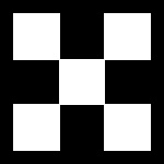 |
square_gaskett_4.dwg 4-th step 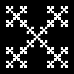 |
square_gasket_8.dwg 8-th step 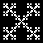 |
You can see the process in animation.
To create this drawing and animation:
Load sierpinski_gasket.lsp (load "sierpinski_gasket")
Then from command line, type square_gasket
Gasket #2
| sqr_gasket2_1.dwg Initial stage 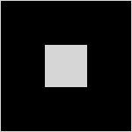 |
sqr_gasket2_2.dwg Second step 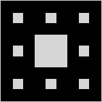 |
sqr_gasket2_4.dwg 4-th step 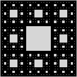 |
sqr_gasket2_7.dwg 7-th step 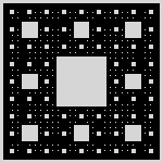 |
You can see the process in animation.
To create this drawing and animation:
Load sierpinski_gasket.lsp (load "sierpinski_gasket")
Then from command line, type square_gasket2
Extension to 3-Dimension:
Cube Gasket
| cube_gasket_1.dwg Initial stage  |
cubee_gasket_2.dwg Second step 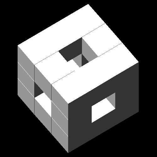 |
cube_gasket_3.dwg 3-rd step 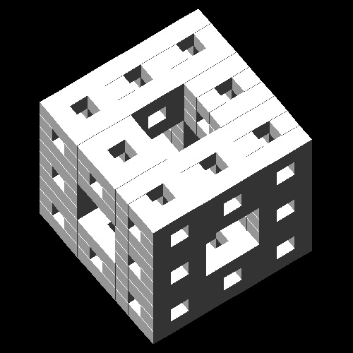 |
cube_gasket_4.dwg 4-th step 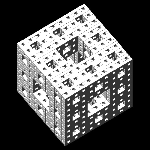 |
cube_gasket_5.dwg 5-th step 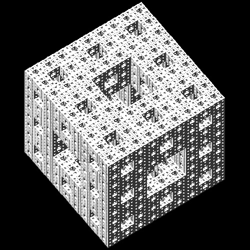 |
You can see the process in animation.
To create this drawing and animation:
Load sierpinski_gasket.lsp (load "sierpinski_gasket")
Then from command line, type cube_gasket
Tetra Gasket
| tetra_gasket_1.dwg Initial stage 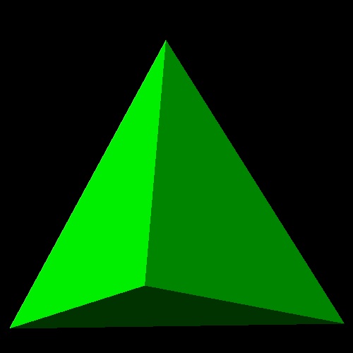 |
tetrae_gasket_2.dwg Second step 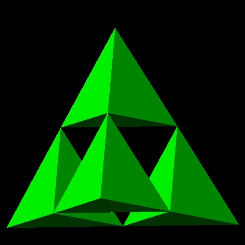 |
tetra_gasket_3.dwg 3-rd step 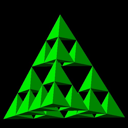 |
tetra_gasket_4.dwg 4-th step 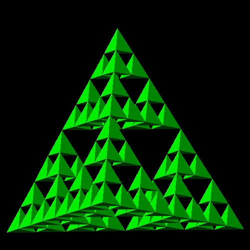 |
tetra_gasket_5.dwg 5-th step 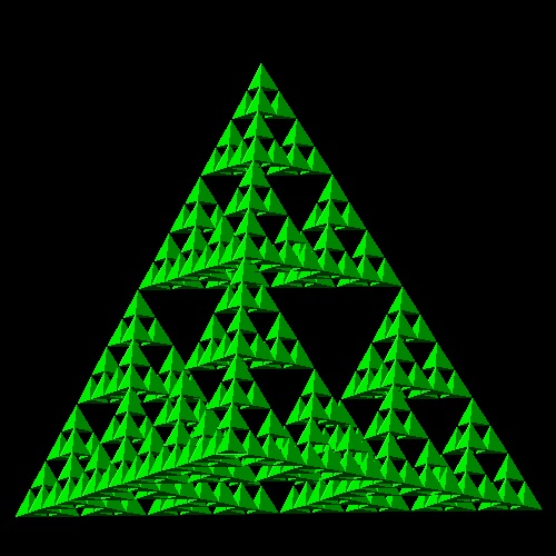 |
You can see the process in animation.
To create this drawing and animation:
Load sierpinski_gasket.lsp (load "sierpinski_gasket")
Then from command line, type tetra_gasket
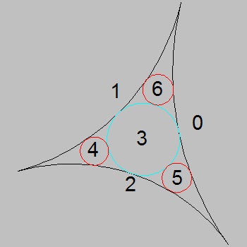
1.5 Leibnitz packing(also called Apollonian gasket or packing)
According to Ref[1], Leibnitz(1646 - 1716) described the circle packing in a letter to de Brosse,
a French aristocrat and writer in 18-th century:
"Imagine a circle;inscribe within it three other circles congruent to each other and of maximum radius;
proceed similarly within each of these circles and within each interval between them,
and imagine that the process continues to infinity..."
The points that were never inside any of the circles form a set of zero area which is more than a line
,but less than a surface.
Its fractal dimension , though its exact value is not known, lies between
1 and 2, approximately 1.3.
If drawing one inside circle tangent to three circles is level-1, then level N is accomplished by
drawing
total sum of {1 + 32 + 33 + ... + 3N-1} circles.
For example , level-9 requires drawing 9841 circles and without computer it is impossible
to draw this many circles.
Examples: From level 2 up to level 9
| circle_fill_level_2.dwg level- 2(4 circles) 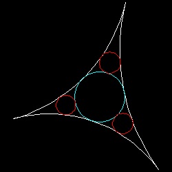 |
circle_fill_level_4.dwg level- 4(40 circles) 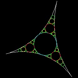 |
circle_fill_level_6.dwg level- 6(364 circles) 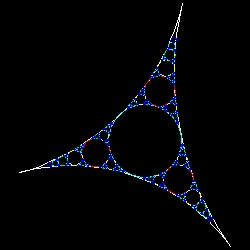 |
circle_fill_level_9.dwg level- 9(9841 circles) 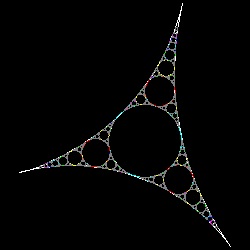 |
You can see the process in animation.
To create this drawing and animation:
First step is to open drawing named test_circle.dwg.
Load circle_fill.lsp (load "circle_fill")
Then from command line, type circle_fill and specify the level of packing.
This program has the option of filling each level of circles with corresponding colors.
This is the example for level-6.
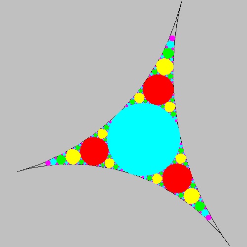
************** level_6_solid.dwg **************
**************** circle_id.dwg ****************
Note: procedure to create these circles
There are two key things to be considered for creating this many circles systematically:First: permutaion list for circles(refer to the figure above right- circle_id.dwg)
If the base 3 arcs are named 0,1,2 as shown, then the first circles to be created is expressed as (0 1 2).
This circle is numbered as 3, then the next 3 circles 4,5 & 6 are designated as (3 1 2), (3 2 0), & (3 0 1).
Then the next level will be (4 1 2), (4 2 3) , (4 3 1) around circle-4, and so on.
So this permultaion list (named as plist in the program) up to level 3 looks like
((0 1 2) (3 1 2) (3 2 0) (3 0 1) (4 1 2) (4 2 3) (4 3 1) (5 2 0) (5 0 3) (5 3 2) (6 0 1) (6 1 3) (6 3 0))
Second: Finding a circle tangent to 3 circles around(Apollonius circle problem)
To draw a circle, a coordinate value of the center (X,Y) and its radius R must be known.
Straight forward method is to solve the following quadratic equations :
(X - xi)2 + (Y - yi)2 = (R + ri)2
for i = 1,2,3
where xi , yi , ri are coordinate values and radii of 3 given circles.
This is the method used here by the author. But radius R can be computed totally independent of the coordinate values
using a very interesting formula found by French mathematician and philosopher René Descartes (1596 - 1650).
2(a2 + b2 +c2 +d2 ) = (a + b + c + d)2
where a,b c & d are the reciprocal of radius (i.e. a = 1/ra, ...) for 4 circles and called "bend".
There is only one formula for eight possible circles, because the bend of a circle can be counted as a negative
if another circle touches it internally.This formula was rediscovered in 1842 and again in 1936 by Sir Frederick Soddy,
the discoverer of Soddy's hexlet.
Test this formula after choosing level 2, and use compute_r4 command.
All the radii (r1,r2,r3) are set to the base circle's radii as default.
The result will match the radius of circle #3.
2. Space Filling curves
2.1 Peano's space filling Curve
| Peano_0.dwg Initial stage 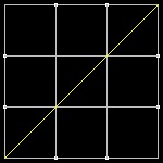 |
Peano_1.dwg Initial stage 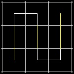 |
Peano_2.dwg First step 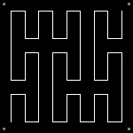 |
Peano_3.dwg Second step 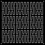 |
| Peano_0.dwg Initial stage |
Peano1_1.dwg 3-rd step 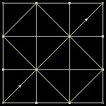 |
Peano1_1.dwg 4-th step 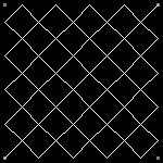 |
Peano1_3.dwg 5-th step 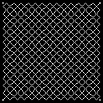 |
| Peano_0.dwg Initial stage |
Peano2_1.dwg 3-rd step 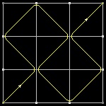 |
Peano2_2.dwg 4-th step 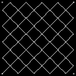 |
Peano2_3.dwg 5-th step 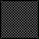 |
Peano curve:
You can see the process in animation.
To create this drawing and animation:
Load Peano.lsp (load "Peano")
Then from command line, type Peano
Peano1 curve:
You can see the process in animation.
To create this drawing and animation:
Load Peano1.lsp (load "Peano1")
Then from command line, type Peano1
Peano2 curve:
You can see the process in animation.
To create this drawing and animation:
Load Peano2.lsp (load "Peano2")
Then from command line, type Peano2
2.2 Hilbert's Space Filling Curves
| Hilbert_0_1.dwg Initial stage 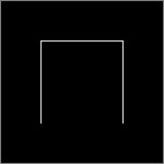 |
Hilbert_0_2.dwg Initial stage 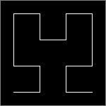 |
Hilbert_0_3.dwg First step 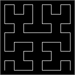 |
Hilbert_0_4.dwg Second step 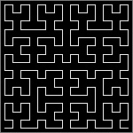 |
| Hilbert_2_0.dwg Initial stage |
Hilbert_2_2.dwg 3-rd step 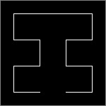 |
Hilbert_2_3.dwg 4-th step 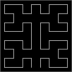 |
Hilbert_2_4.dwg 5-th step 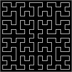 |
| Hilbert_3_1.dwg Initial stage 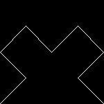 |
Hilbert_3_2.dwg 3-rd step 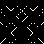 |
Hilbert_3_3.dwg 4-th step 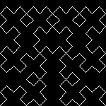 |
Hilbert_3_4.dwg 5-th step 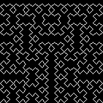 |
| Hilbert_4_1.dwg Initial stage 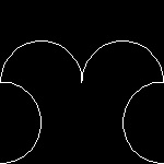 |
Hilbert_4_2.dwg 3-rd step 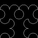 |
Hilbert_4_3.dwg 4-th step 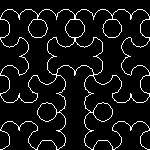 |
Hilbert_4_4.dwg 5-th step 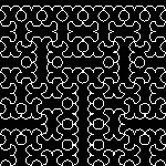 |
Hilbert's curve #1: You can see the process in animation.
To create this drawing and animation:
Load Hilbert1.lsp (load "Hilbert")
Then from command line, type Hilbert
Hilbert's curve #2:
You can see the process in animation.
To create this drawing and animation:
Load Hilbert2.lsp (load "Hilbert2")
Then from command line, type Hilbert2
Hilbert's curve #3:
You can see the process in animation.
To create this drawing and animation:
Load Hilbert3.lsp (load "Hilbert3")
Then from command line, type Hilbert3
Hilbert's curve #4:
You can see the process in animation.
To create this drawing and animation:
Load Hilbert4.lsp (load "Hilbert4")
Then from command line, type Hilbert4
2.3 Sierpinski's Space Filling Curves
| Sierpinski_0_0.dwg Initial stage 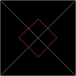 |
Sierpinski_0_1.dwg Initial stage 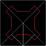 |
Sierpinski_0_2.dwg First step 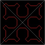 |
Sierpinski_0_3.dwg Second step 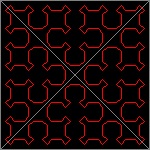 |
| Sierpinski_1_0.dwg Initial stage 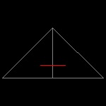 |
Sierpinski_1_1.dwg Initial stage 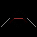 |
Sierpinski_1_2.dwg First step 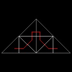 |
Sierpinski_1_3.dwg Second step 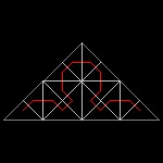 |
Sierpinski's Space filling curve: You can see the process in animation.
To create this drawing and animation:
Load Sierpinski.lsp (load "Sierpinski")
Then from command line, type Sierpinski
2.4 Levy's "C-shape" curve
| c_shape1_1.dwg Initial stage  |
c_shape1_2.dwg 2-nd stage 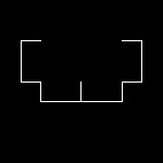 |
c_shape1_3.dwg 3-rd step  |
c_shape1_4.dwg 4-th step  |
c_shape1_5.dwg 5-th step  |
| c_shape2_1.dwg Initial stage  |
c_shape2_2.dwg 2-nd stage  |
c_shape2_3.dwg 3-rd step 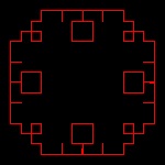 |
c_shape2_4.dwg 4-th step 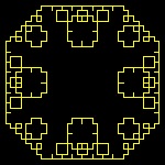 |
c_shape2_5.dwg 5-th step 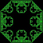 |
| c_shape3_1.dwg Initial stage 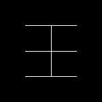 |
c_shape3_2.dwg 2-nd stage 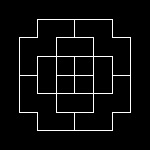 |
c_shape3_3.dwg 3-rd step 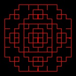 |
c_shape3_4.dwg 4-th step 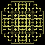 |
c_shape3_5.dwg 5-th step 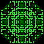 |
To create this drawing and animation:
Load c_shape.lsp (load "c_shape")
Then from command line, type c_shape1, c_shape2, & c_shape3
3. Fractal Tree, Dragon curves
3.1 Fractal Trees (ref . ??)
| fractal_tree_2.dwg 2-nd stage 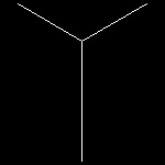 |
fractal_tree_4.dwg 4-th stage 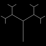 |
fractal_tree_6.dwg 6-th stage 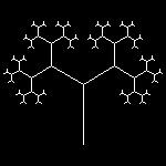 |
fractal_tree_9.dwg 9-th stage 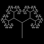 |
fractal_tree.dwg final step 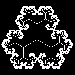 |
| tree_lune_2.dwg Initial stage  |
tree_lune_4.dwg 2-nd stage 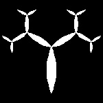 |
tree_lune_6.dwg 3-rd step 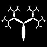 |
tree_lune_9.dwg 4-th step 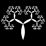 |
fractal_tree_lune.dwg 5-th step 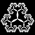 |
| tree_trig_2.dwg 2-nd stage 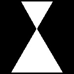 |
tree_trig_4.dwg 4-th stage 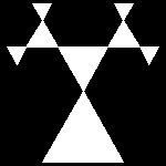 |
tree_trig_6.dwg 6-th step 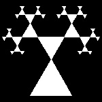 |
tree_trig_9.dwg 9-th step 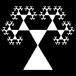 |
fractal_tree_trig.dwg final stage 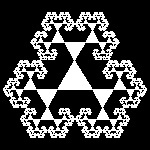 |
| tbranch_2.dwg Initial stage 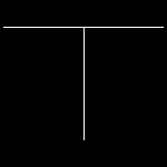 |
tbranch_4.dwg 2-nd stage 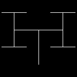 |
tbranch_6.dwg 3-rd step 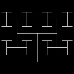 |
tbranch_9.dwg 4-th step 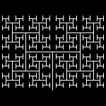 |
fractal_tbranch.dwg 5-th step 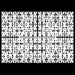 |
| tbranch_square_2.dwg Initial stage  |
tbranch_square_4.dwg 2-nd stage  |
tbranch_square_6.dwg 3-rd step 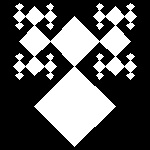 |
tbranch_square_8.dwg 4-th step 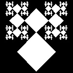 |
fractal_tbranch_square.dwg 5-th step 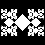 |
| 3fold_2.dwg Initial stage  |
3fold_4.dwg 2-nd stage 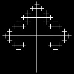 |
3fold_6.dwg 3-rd step 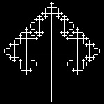 |
3fold_8.dwg 4-th step 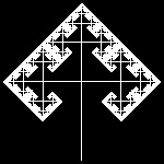 |
fractal_3fold.dwg 5-th step 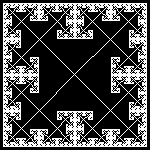 |
| 3fold_lune_2.dwg 2nd stage  |
3fold_lune_4.dwg 4-th stage  |
3fold_lune_5.dwg 5-th step  |
3fold_lune_6.dwg 6-th step  |
fractal_3fold_lune.dwg final step 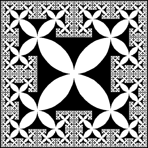 |
| 3fold_square_2.dwg 2-nd stage  |
3fold_square_4.dwg 4-th stage  |
3fold_square_6.dwg 6-th step 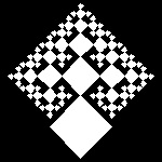 |
3fold_square_7.dwg 7-th step 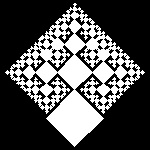 |
fractal_3fold_square.dwg final step 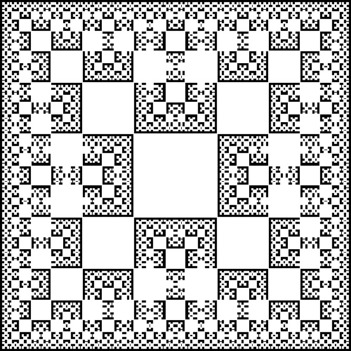 |
| pent_2.dwg 2nd stage 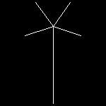 |
pent_4.dwg 4-th stage 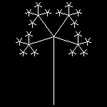 |
pent_5.dwg 5-th step 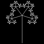 |
pent_6.dwg 6-th step 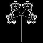 |
fractal_pent.dwg final step 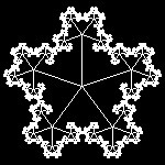 |
| pent_lune_2.dwg 2-nd stage  |
pent_lune_4.dwg 4-th stage 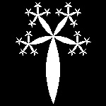 |
pent_lune_5.dwg 5-th step 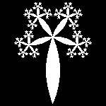 |
pent_lune_6.dwg 6-th step 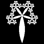 |
fractal_pent_lune.dwg final step 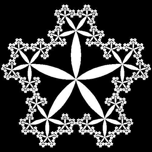 |
| pentagon_2.dwg 2-nd stage 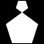 |
pentagon_4.dwg 4-th stage 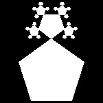 |
pentagon_5.dwg 5-th step 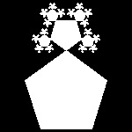 |
pentagon_6.dwg 6-th step 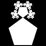 |
fractal_pentagon.dwg final step 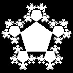 |
| pentagon_whole_2.dwg 2-nd stage 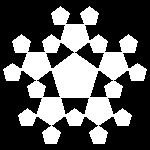 |
pentagon_whole_4.dwg 4-th stage 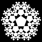 |
pentagon_whole_5.dwg 5-th step 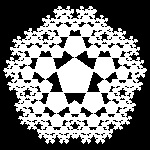 |
pentagon_whole_6.dwg 6-th step 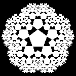 |
fractal_pentagon_whole.dwg 7-th step 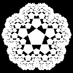 |
To create this drawing and animation:
Load fractal_tree.lsp (load "fractal_tree")
case: command & Input
tree: tree,input(golden ratio=0.618043)
tree_lune: tree_lune,input(golden ratio=0.618043)
tree_trig: tree_trig,input(golden ratio=0.618043)
tbranch: tbranch,input(golden ratio=0.618043)
tbranch_square: tbranch_square,input(golden ratio=0.618043)
3fold: 3fold,input(0.5)
3fold_lune: 3fold_lune,input(0.5)
3fold_square: 3fold_square,input(golden ratio=0.618043)
pent: pent,input(one_m_rho)
pent_lune: pent_lune,input(one_m_rho)
pentagon: pentagon,input(one_m_rho)
pentagon_whole: pentagon_whole,input(golden ratio=0.618043)
3.2 Pythagoras Tree (ref . ??)
| ptree_1_1.dwg 1-st stage 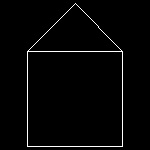 |
ptree_1_3.dwg 3-rd stage 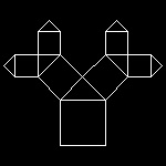 |
ptree_1_6.dwg 6-th stage 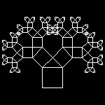 |
ptree_1_8.dwg 8-th stage 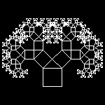 |
ptree_1_13.dwg 13-th stage 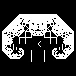 |
| ptree_2_1.dwg 1-st stage 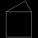 |
ptree_2_3.dwg 3-rd stage 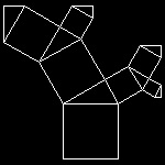 |
ptree_2_6.dwg 6-th stage 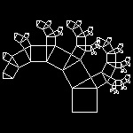 |
ptree_2_8.dwg 8-th stage 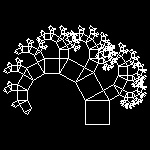 |
ptree_2_13.dwg 13-th stage 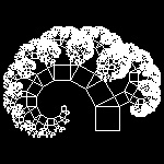 |
| ptree_3_1.dwg 1-st stage 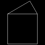 |
ptree_3_3.dwg 3-rd stage 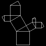 |
ptree_3_6.dwg 6-th stage 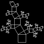 |
ptree_3_8.dwg 8-th stage 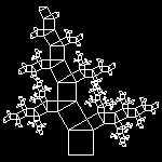 |
ptree_3_13.dwg 13-th stage 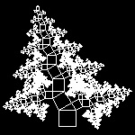 |
| linetree1_1.dwg 1-st stage 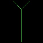 |
linetree1_3.dwg 3-rd stage 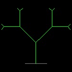 |
linetree1_6.dwg 6-th stage 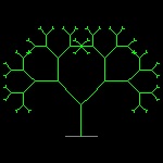 |
linetree1_8.dwg 8-th stage 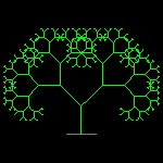 |
linetree1_11.dwg 11-th stage 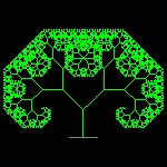 |
| linetree3_1.dwg 1-st stage 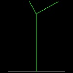 |
linetree3_3.dwg 3-rd stage 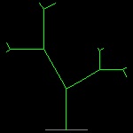 |
linetree3_6.dwg 6-th stage 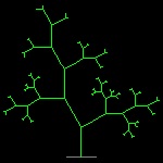 |
linetree3_8.dwg 8-th stage 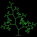 |
linetree3_12.dwg 12-th stage 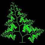 |
| linetree2_1.dwg 1-st stage  |
linetree2_3.dwg 3-rd stage 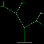 |
linetree2_6.dwg 6-th stage 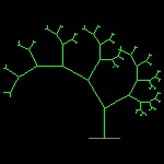 |
linetree2_8.dwg 8-th stage 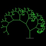 |
linetree2_12.dwg 12-th stage 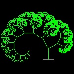 |
| tree3_fill_1.dwg 1-st stage  |
tree3_fill_3.dwg 3-rd stage  |
tree3_fill_6.dwg 6-th step 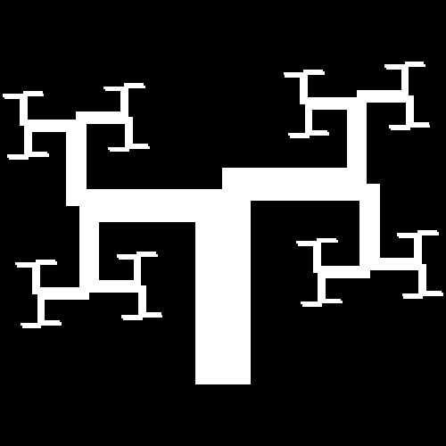 |
tree3_fill_8.dwg 8-th step 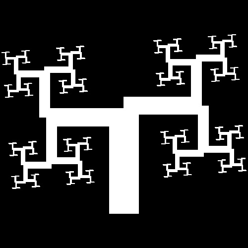 |
tree3_fill_10.dwg 10-th step 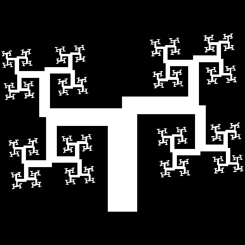 |
| tree4_fill_1.dwg 1-st stage  |
tree4_fill_3.dwg 3-rd stage 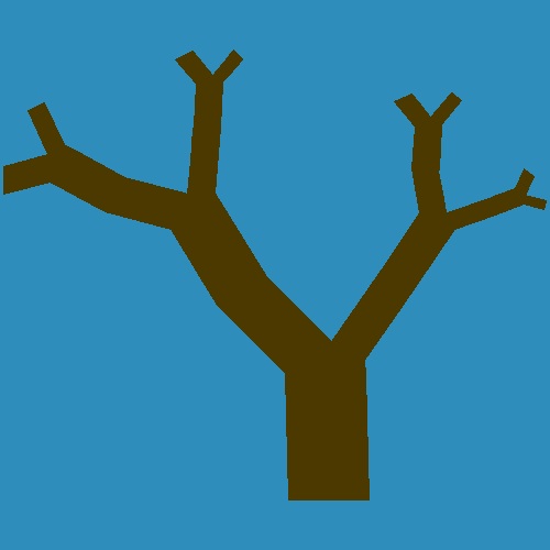 |
tree4_fill_6.dwg 6-th step  |
tree4_fill_8.dwg 8-th step  |
tree4_fill_11.dwg 11-th step  |
| tree5_1.dwg 1-st stage  |
tree5_3.dwg 3-rd stage 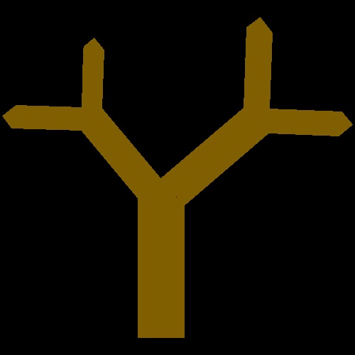 |
tree5_6.dwg 6-th step  |
tree5_8.dwg 8-th step  |
tree5_12.dwg 11-th step  |
To create this drawing and animation:
Load pythagoras_tree.lsp (load "pythagoras_tree")
Executable:
pythagorean_tree
tree2
tree3
tree4
tree5
3.2 Dragon Curves (ref . ??)
| page50_1.dwg Initial stage  |
page50_2.dwg 2-nd stage  |
page50_3.dwg 3-rd stage  |
page50_4.dwg 4-th stage 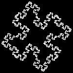 |
page50_5.dwg 5-th step 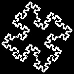 |
| page52_1.dwg Initial stage  |
page52_2.dwg 2-nd stage 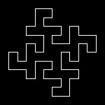 |
page52_3.dwg 3-rd stage 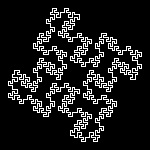 |
page52_4.dwg 4-th stage 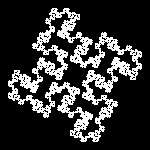 |
page52_5.dwg 5-th step 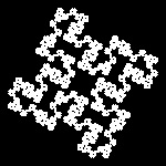 |
| page54_1.dwg Initial stage  |
page54_2.dwg 2-nd stage 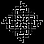 |
page54_3.dwg 3-rd stage 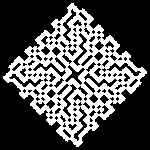 |
page54_3.dwg 3-rd stage detail 1 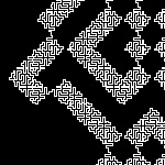 |
page54_3.dwg 3-rd stage detail 2 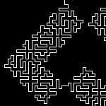 |
| page55_1.dwg Initial stage  |
page55_2.dwg 2-nd stage 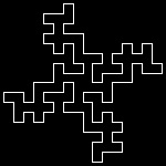 |
page55_3.dwg 3-rd stage 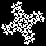 |
page55_3.dwg 3-rd stage detail 1 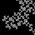 |
page55_3.dwg 3-rd stage detail 2 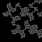 |
| page64_1.dwg Initial stage 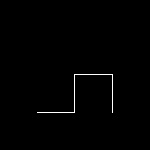 |
page64_2.dwg 2-nd stage 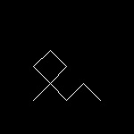 |
page64_6.dwg 6-th stage 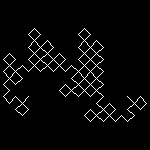 |
page64_10.dwg 10-th stage 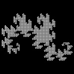 |
page64_14.dwg 14-th stage 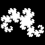 |
| page68_1.dwg Initial stage 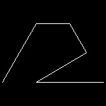 |
page68_2.dwg 2-nd stage 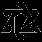 |
page68_4.dwg 4-th stage 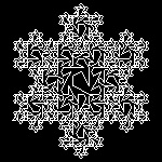 |
page68_4_round.dwg 4-th step rounded 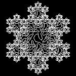 |
page68_4_round.dwg 4-th step detail  |
| page70_1.dwg Initial stage 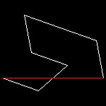 |
page70_2.dwg 2-nd stage 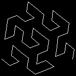 |
page70_3.dwg 3-rd stage 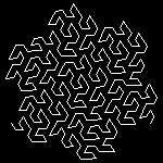 |
page70_4.dwg 4-th step 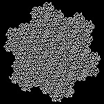 |
page70_4_det.dwg 4-th step detail 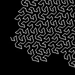 |
To create this drawing and animation:
Load fractal_mandelb.lsp (load "fractal_mandelb")
Then from command line, type page50, 52, 54,...,70
4. Function Iteration and Newton's method
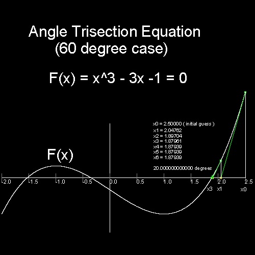
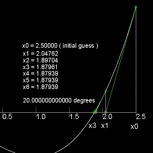
4.1 Newton's method
| newton1_result.dwg
newton1_result.jpg Funtion Graph 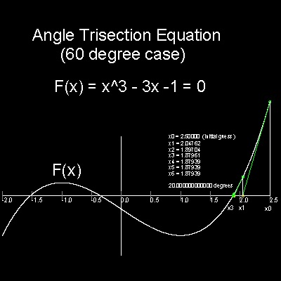 |
newton1_result.dwg
newton1_result_detail.jpg Process Detail 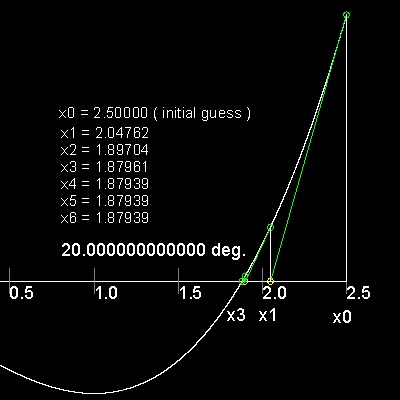 |
To create this drawing :
Load newton1.lsp (load "newton1")
Then from command line, type newton1
But this method works only if the function graph f(x) has point(s) of intersection on x-axis.
For example, when f(x) = x2 + 1 = 0, this method does not work !!
Cayley proposed that if this idea is expanded to the complex plane (z = x + iy), then it is possible to obtain the roots in the complex plane, and he showed one example in a quadratic equation case.
4.2 iteration of quadratic functions
Function tested is given by f(z) = z2 + 1 = 0. Since f', ( firrst derivative of f(z) ) = 2z, the iteration function is:zn+1 = (1/2)(zn - 1/zn)
Orbit test
First let us find out the general behaviour of the iteration function used .The iteration function is given by zn+1 = (1/2)(zn - 1/zn)
The process goes this way:
Select any point in the complex plane. This is the initial guess point(z0).
Compute z1 using the iterationn function. Connect z0 and z
Continue the process 10 times. Color the point z0, white, z1, red, z2, yellow, z3, green,etc for clear identification.
After several steps all points converge to one of the two roots.
The result is shown below.
To create this drawing :
Load fractal_tools.lsp (load "fractal_tools")
Then from command line, type orbit_test_f4
| orbit_test_quadratic.dwg orbit_test_quadratic.jpg Orbit Test 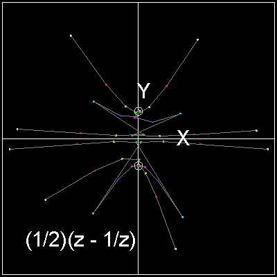 |
orbit_test_quadratic.dwg orbit_test_quadratic_detail.jpg Orbit Test -detail 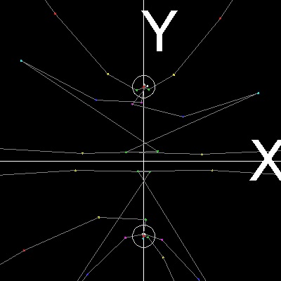 |
| newton_quadratic_1.dwg
newton_quadratic_1.jpg Color map1 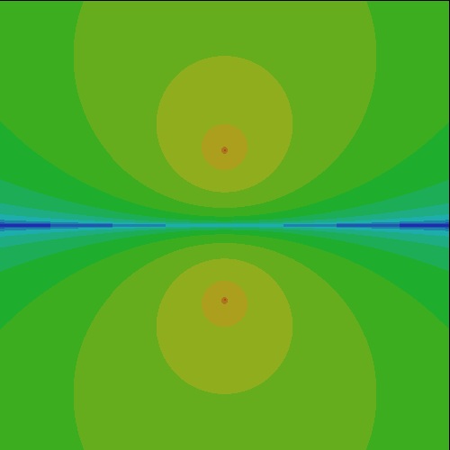 |
newton_quadratic_1.dwg
newton_quadratic_2.jpg Color map2 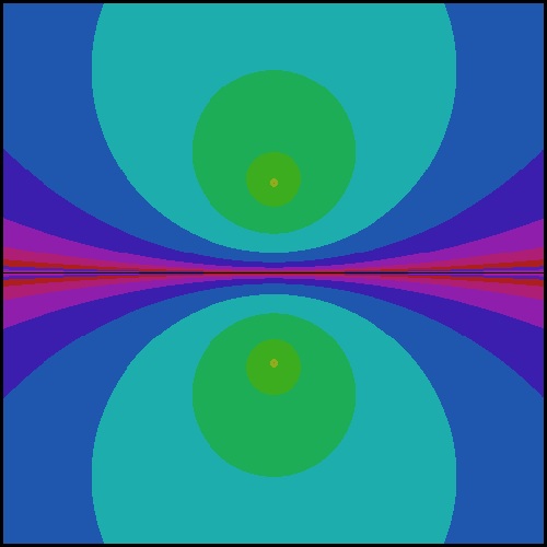 |
newton_quadratic_1.dwg
newton_quadratic_3.jpg Color map3 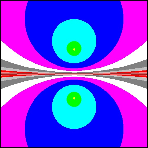 |
To create this drawing :
Load newton_iteration.lsp (load "newton_iteration")
Then from command line, type quadratic
Now it looks easy to apply the same idea to the case of cubic equation.
4.3 iteration of cubic equation
Function tested is given by f(z) = z3 - 1 = 0. Since f', ( first derivative of f(z) ) = 3z2, the iteration function is:zn+1 = (2 (zn)3 + 1)/(3(zn)2)
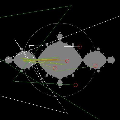
Orbit test
First let us find out the general behaviour of the iteration function used .The iteration function is given by zn+1 = (2 (zn)3 + 1)/(3(zn)2)
The process goes this way:
Select any point in the complex plane. This is the initial guess point(z0).
Compute z1 using the iterationn function. Connect z0 and z
Continue the process 20 times. Color the point z0, white, z1, red, z2, yellow, z3, green,etc for clear identification.
After several steps all points converge to one of the three roots.
The result is shown below.
To create this drawing :
Load fractal_tools.lsp (load "fractal_tools")
Then from command line, type orbit_test_f5
| orbit_test_cubic.dwg orbit_test_cubic.jpg Orbit Test 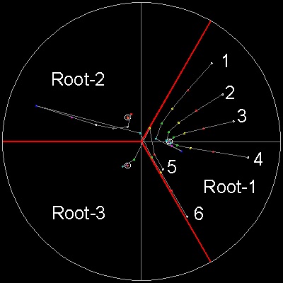 |
orbit_test_cubic.dwg orbit_test_cubic_detail.jpg Orbit Test -detail 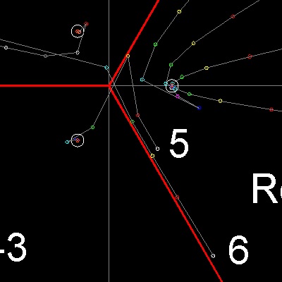 |
In this drawing, 3 thick red lines divides whole complex plane into 3 regions, each corresponding to the root within the region.
Our intuition tells us that any point selected in the region, after iterations, would converge to the root within the region
where the point belongs.
Orbit test result shows otherwise. Points 1-4 behaves as expected, but points 5,6 converge to the root in other regions.
In order to see the behaviour, the same algorith is used to compute iteration map for this cubic equation.
The result is shown below. Obviously something complex is happening around the boundary regions.(See color map 1)
Since this map does not distinguish which root the particular point is converging, another algorithm is used to color the points
according to the roots the iteration ends up.
The points ,which eventually converge to root-1 (1,0), is colored with Red Hue.
Root-2 uses Green Hue, and Root-3, Blue Hue.(See color map 2)
This will explain clearly what is happening to point 5,6 in orbit test.
Click here to see Cubic Iteration Solution animation
| newton_cube_50_1.dwg
newton_cube_50_1.jpg Color map1 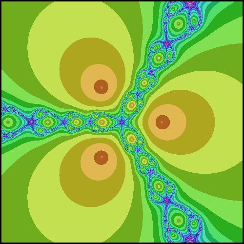 |
cubic_newton_10.dwg
cubic_newton_10.jpg Color map2 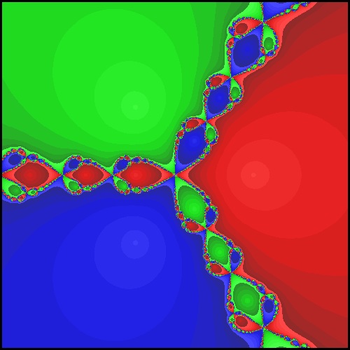 |
cubic_newton_22.dwg
cubic_newton_22.jpg Color map3 (Detail) 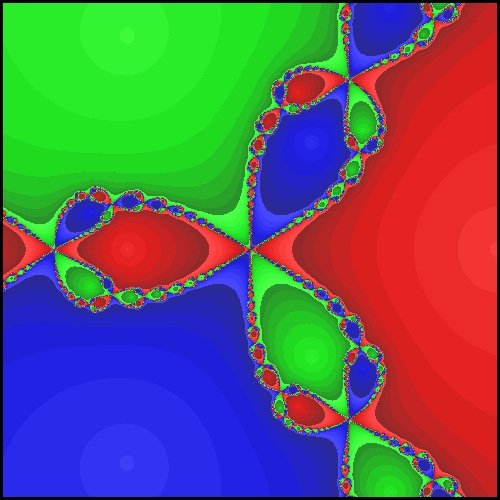 |
To create this drawing :
Load newton_iteration.lsp (load "newton_iteration")
Additional step:
Load fractal_tools.lsp (load "fractal_tools")
Color map 1
Then from command line, type cubic_1
For coloring nodes, use LAYER_COLOR_TEST command.
For the following 2 cases, use SET_NEWTON_COLOR1 command.
Color map 2
Then from command line, type cubic_rgb
Color map 3
Then from command line, type cubic_autozoom
This is the 22-nd picture of the series.
4.4 iteration of quintic equation
Function tested is given by f(z) = z5 - 1 = 0.Since f', ( first derivative of f(z) ) = 5z4, the iteration function is: zn+1 = (4 (zn)5 + 1)/(5(zn)4)
The typical results are shown below.
Map 1 uses the basic 5 colors with changing light index, and Map2 & 3 uses command SET_QUINTIC_COLOR.
| newton_z5-5colors.dwg newton_z5-5colors.jpg Color map1 range (-1 -1) ~ (1,1) 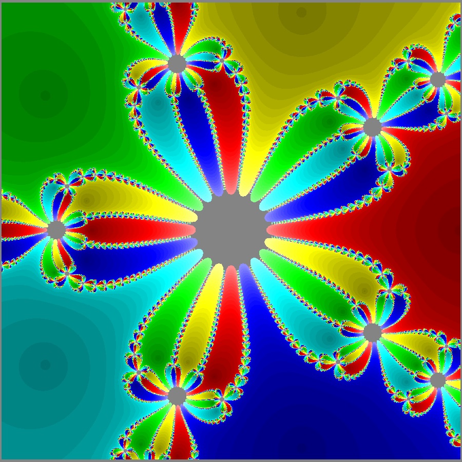 |
quintic_1.5x1.5.dwg
quintic_1.5x1.5.jpg Color map2 (-1.5,-1.5) ~ (1.5,1.5)  |
quintic_1x1_40.dwg
quintic_1x1_40.jpg Color map3 (-1,-1) ~ (1,1) |
To create this drawing :
Load newton_iteration.lsp (load "newton_iteration")
Additional step:
Load fractal_tools.lsp (load "fractal_tools")
Color map 1
Then from command line, type quintic
For coloring nodes, use LAYER_COLOR_TEST command.
For the following 2 cases, use SET_quintic_color command.
Color map 2 & 3
Then from command line, type quintic
5. Julia Set
The simplest example is quadratic function z2 .Choose any complex number z = x + iy,which represents coordinate value (x,y) in Cartesian coordinate system, and a complex constant c. A quadratic function f(z) = z2 + c is used to caluculate the sequential location of z. Repeat the process and the resulting position of z is plotted on the x-y plane.
What will be the result ?
There are 3 possibilities for the point selected:
(1) it may go further and further away from the initial point and disappear toward infinity.
(2) it may tend toward a fixed point
(3) it may jump around in a region (called "strange attractor")
| orbit_test_1.dwg orbit_test_1.jpg Orbit Test 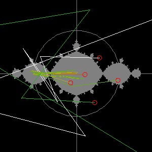 |
| orbit_test_scene_1.dwg
orbit_test_scene_1.jpg C = -1  |
orbit_test_scene_2.dwg
orbit_test_scene_2.jpg C = 0.3 - 0.4 i 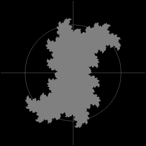 |
orbit_test_scene_3.dwg
orbit_test_scene_3.jpg C = .360284 + .100376 i 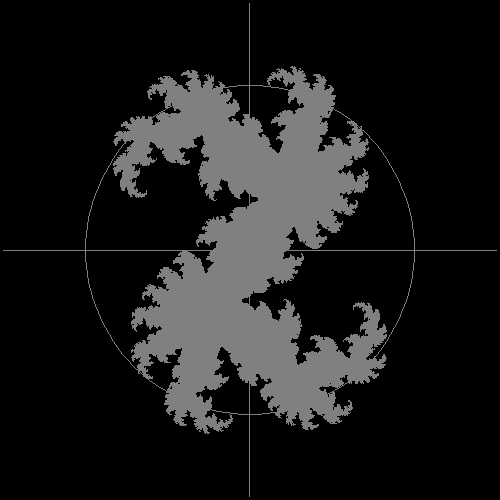 |
orbit_test_scene_4.dwg
orbit_test_scene_4.jpg C = -.1 + .8 i 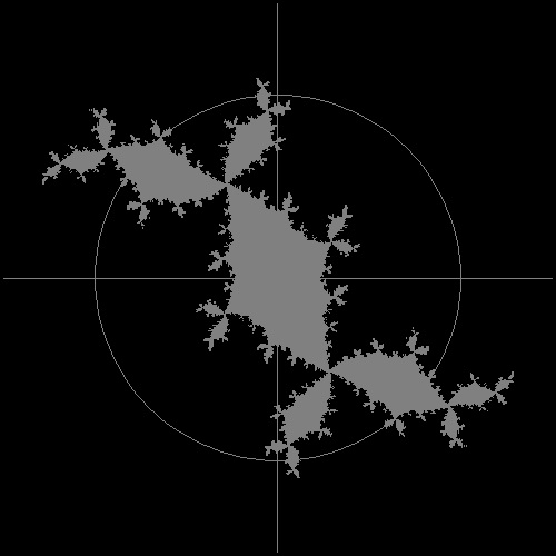 |
There are only two types of Julia set depending upon the location of "k" .
They are either connected or disconnected like Cantor set(called Fatou dust).
It is easy to understand the situation if the simplest case is considered.
5.1 Julia Set for a quadratic function ( z2 + c )
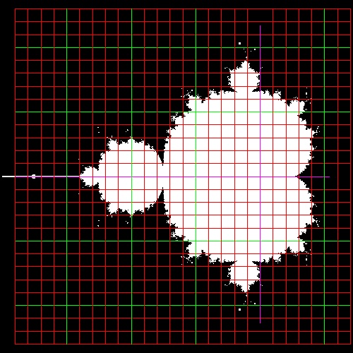
In this case, "connected" or "disconnected" is decided by where the point "c" is located in the Mandelbrot SetMandelbrot set will be discussed next, but for now, let us say there is a map which explains the behaviour of Julia set, and this is called mandelbrot Set.
Julia_set_sample_data_location.dwg
*** Click the frame to see full picture ***
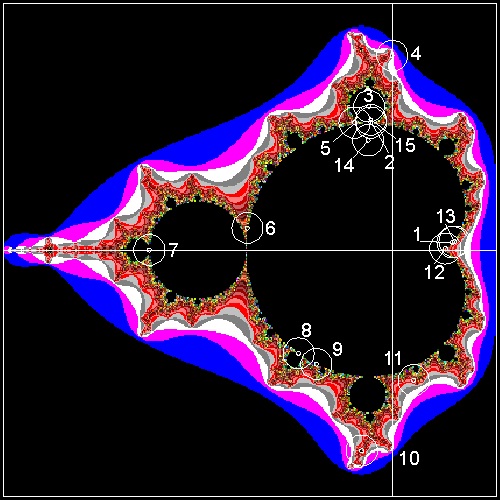
Data Set ID No.			C value				Range
			Real		Imag
	1		0.31		0.04		(1.0486 1.3135)
	2		-0.11		0.6557		(1.3982 1.2157)
	3		-0.12		0.74		(1.3842 1.2017)
	4		0.0		1.0		(1.4261 1.2716))
	5		-0.194		0.6557		(1.5799 0.9921)
	6		-0.74543	0.11301    	(1.5391 0.9100)
	7		-1.25		0.0		(1.7748 0.7825)
	8		-0.481762	-0.531657	(1.5100 1.0900)
	9		-0.39054	-0.58679   	(1.4821 1.1179)
	10		-0.15652	-1.03225   	(1.4681 1.2157)
	11		0.11031		-0.67037   	(1.3003 1.2576)
	12		0.27334		0.00742		(1.0626 1.2716)
	13		0.32		0.043		(0.85821 1.12914)
	14		-0.12375   	0.56508		(1.5 1.5)
	15		-0.11		0.67		(1.5 1.5)
Mono-chrome output
Mathematically speaking, Julia set is a set of points which do not approach infinityafter so many iterations. But for convenience , the iteration number is set as 100.
If the test point satisfy the condition for Julia Set, then the point is colored white.
The example run for case ID # 1 is shown below.
Two different algorithms are used here:
Algorithm A: If iteration exceeds 100, then color the point white and go to next test point.
Algorithm B: If iteration exceeds 30, and does not exceeds 100, color the point according to the
predefined rule, and go to the next point.
"A" will create the filled up map like the one in the left below. This is the true definition of Julia Set,
but the drawing file size becomes big.
"B" will create a boundary like map of the filled-set, and the drawing size is much smaller.
How to run Algorith A program :
Load julia_mono_filled.lsp (load "julia_mono_filled")
Then from command line, type julia_mono_filled
How to run Algorith B program :
Load julia_mono_test.lsp (load "julia_mono_test")
Then from command line, type julia_mono_test
|
julia_case_1_filled.dwg julia_case_1_filled.jpg Case #1 Filled 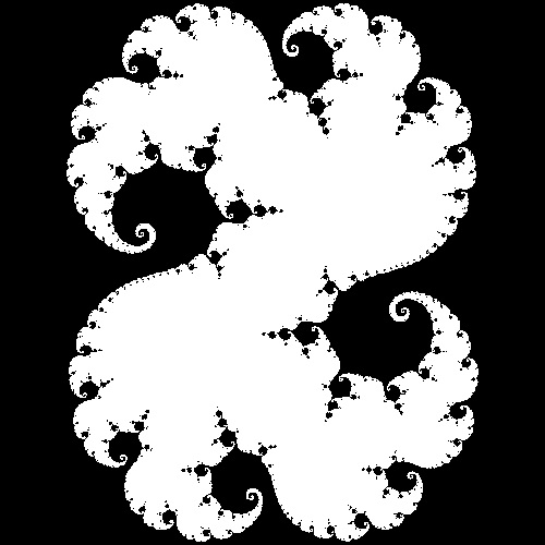 |
Julia_01_002_mono2.dwg Julia_01_002_mono2.jpg Case #01 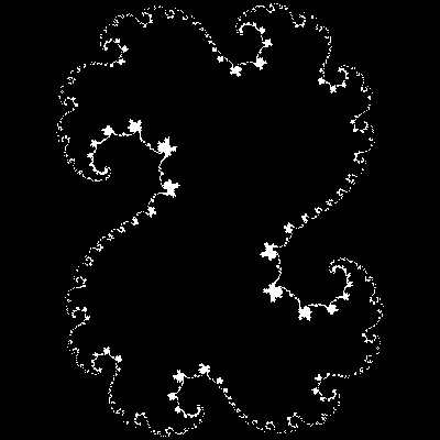 |
The following 12 drawings are created using Algorithm B.
How to create the following mono-chrome drawings :
Load julia_mono_test.lsp (load "julia_mono_test")
Then from command line, type julia_mono_test
Input data exmaple for case ID #1
Command: julia_mono_test

Specify the requested set(def=1)			Return Key for Default set
Spacing = (def = 0.01)					0.002
Starting point (def = data from pre-defined list))	Return Key for Default set
Ending point (def = data from pre-defined list)		Return Key for Default set
-1.3135		These are y coordinate value now being processed
-1.3115
-1.3095
|
Julia_01_002_mono2.dwg #01: 0.31 , 0.34 |
Julia_02_002_mono2.dwg #02: -0.11, 0.6557 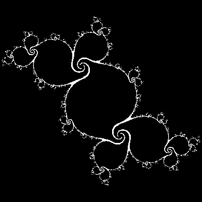 |
Julia_03_002_mono2.dwg #03: -0.12, 0.74 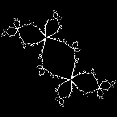 |
Julia_04_mono_a.dwg #04: 0.0 , 1.0  |
Julia_05_mono_001.dwg #05: -0.194 , 0.6557  |
|
Julia_06_mono9.dwg #06: -0.7454 , 0.1130  |
Julia_07_mono.dwg #07: -1.25 , 0.0  |
Julia_08_mono.dwg #08: -0.4818, -0.5317  |
Julia_09_mono.dwg #09: -0.3905, -0.5868  |
Julia_10_mono.dwg #10: -0.1565, -1.0322  |
|
Julia_11_mono.dwg #11: 0.1103, -0.6703  |
Julia_12_mono.dwg #12: 0.2733, 0.0074  |
Julia_13_mono.dwg #13: 0.32, 0.043  |
Julia_14_mono_005.dwg #14: -0.1238, 0.5651  |
Julia_15_mono.dwg #15: -0.11, 0.6703  |
Note:Case #14 is created differently from other 14 cases.
Steps taken are as follows:
(1) create filled julia set using :JULIA_MONO_FILLED" in julia_mono_filled.lsp
(2) Then use executable "FILLED_TO_BSM" in fractal_tools.lsp to eliminate the inside points.
The algorith used is called "Boundary Search Method" (BSM).
How to create the following colored drawings :
Algorithm used to create colored maps is the same as the one used for Mono-chrome case except
that when the test point diverge, the point is painted with a color assigned to the iteration number.
For example , one point goes outside the radius = 2 circle after n iteration, that point is
assigned a color unique to the number "n".
In addition to loading my_tools.lsp, fractal_tools.lsp must be loaded for all the following
execution.
Load fractal_tools.lsp (load "fractal_tools")
Load julia_set.lsp (load "julia_set")
Then from command line, type julia_set
When the program is run, there are 6 input prompts.
Here is an example input for case ID #1.
When Default Input is OK, just hit the return key to accept the default value.
Note: Screensize is set to 500 x 500 pixels in AutoCAD graphic screen.

Command: julia_set

(1) Specify the requested set(def=1)
(2) Starting point (def = data from pre-defined list))
(3) Ending point (def = data from pre-defined list)

(4) Minimum iteration = (def=1)5

(5) Maximum iteration = (def=100)200
		default spacing = 0.00444
(6) Spacing = (def = dx/500.)
Color output
|
Julia_01_002_color.dwg Case #01 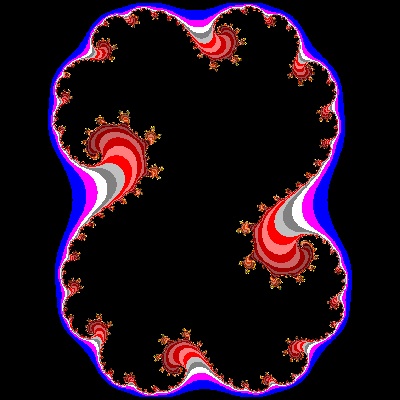 |
Julia_02_002_color.dwg Case #02 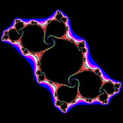 |
Julia_03_002_color.dwg Case #03 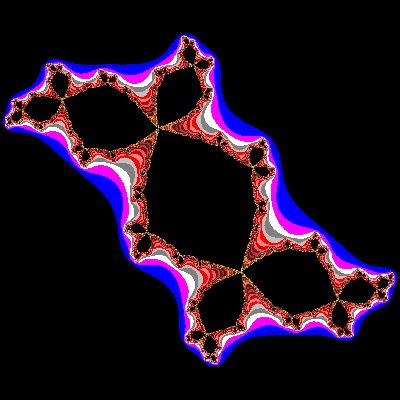 |
Julia_04_002_color.dwg Case #04 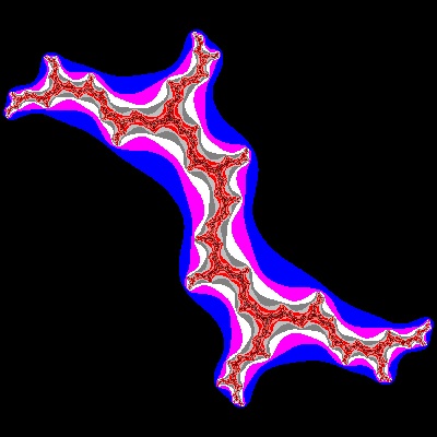 |
Julia_05_002_color.dwg Case #05 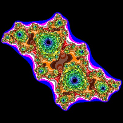 |
|
Julia_06_002_color.dwg Case #06 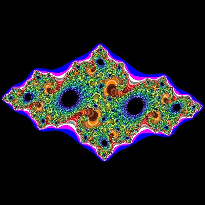 |
Julia_07_002_color.dwg Case #07 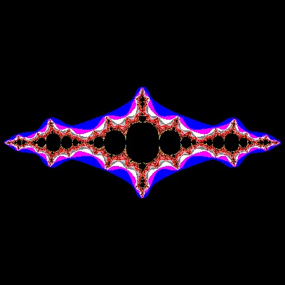 |
Julia_08_001_color.dwg Case #08 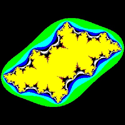 |
Julia_09_002_color.dwg Case #09 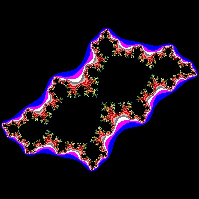 |
Julia_10_002_color.dwg Case #10 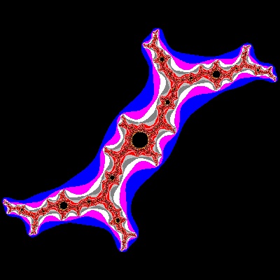 |
|
Julia_11_002_color.dwg Case #11 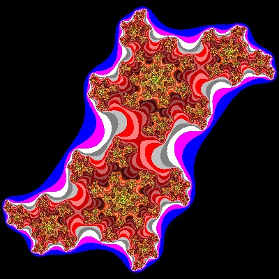 |
Julia_12_002_color.dwg Case #12 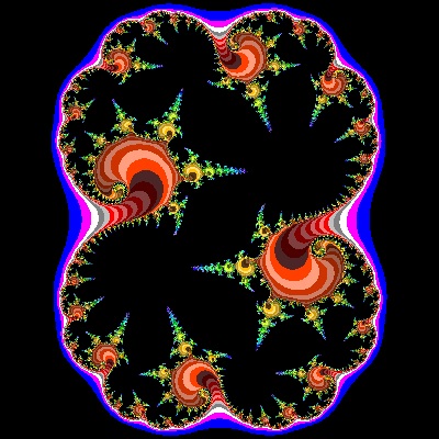 |
Julia_13_001_color.dwg Case #13 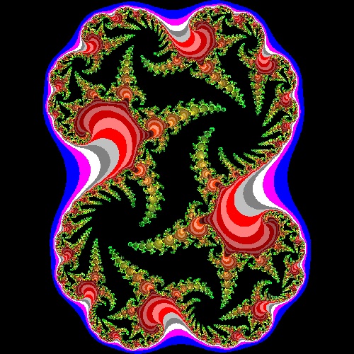 |
Julia_14_002_color.dwg Case #14 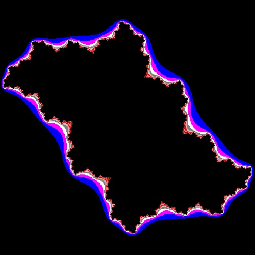 |
Julia_15_002_color.dwg Case #15 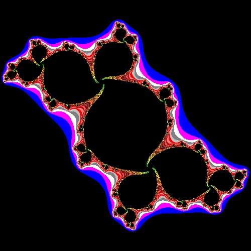 |
5.2 Julia-like fractal for other functions
In order to create Julia-like color map by iterating other analytic functions,it is helpfull to derive sine, cosine, exponential , and hyperbolic-sine & cosine functions
for complex value z = x + i y .
	Begin with the following Euler's equation:
		e i z  =  cos z  + i sin z
	From this we derive the further relations:
		cos z = (eiz + e-iz)/ 2
			sin z = (eiz - e-iz)/ (2 i)
	For purely imaginary z, z = iy, this relation give
		cos iy = (ey + e-y)/2 = cosh y
		sin iy = (ey - e-y)/(2 i) = i sinh y
   Using the above relations, we can now write the following relations
   in real and imaginary part.

   cosz & sinz:
	With the help of the addition theorems of trigonometry,
		cos z = cos(x + iy) = cosx coshy - i sinx sinhy
		sin z = sin(x + iy) = sinx coshy + i cosx sinhy
   ez:
		ez = ex + iy = ex eiy
		   =  ex(cos y + i sin y)
   cosh z:
		cosh z = (ez + e-z)/2 = coshx cosy + i sinhx siny

   sinh z:
		sinh z = (ez - e-z)/2 = sinhx cosy + i coshx siny

   Note: Escape criteria:
	trigonometric functions: Absolute value of its "Imaginary" part > 50
	exponential function: Absolute value of its "Real" part > 50
5.2 Sine, Cosine and Exponential functions
Global pictures:Function mapping range --------------------------------------------------- Sine : z:-> sin(z) (-5,-5) (5,5) Cosine : z:-> cos(z) (-5,-5) (5,5) Exponenential : z:-> exp(z) (-4,-4) (4,4) Maximum iteration = 50Click a mouse on the picture for a larger image.
|
julia_sine_global.dwg Sine Function-frame size 10 x 10 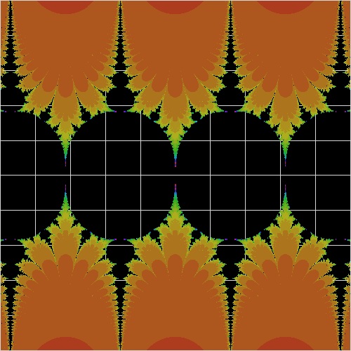 |
julia_cosine_global.dwg Cosine function - frame size 10 x 10 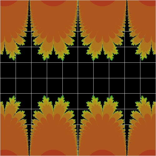 |
julia_exp_global.dwg Exponential - frame size 8 x 8 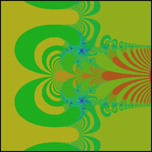 |
5.2.1 Complex Sine function
    The iterated function is of the form  z:-> k sine(z)
		where z = x + iy, and k = R + i I
    The results are shown for the following cases:
    (1) Pure real case: I = 0
    (2) Pure imaginary case: R = 0
    (3) when k = a + ib
    (4) when k = 1 + ib (real part is equal to 1)
How to create the following colored drawings :
In addition to loading my_tools.lsp, fractal_tools.lsp must be loaded for all the following execution.
Load fractal_tools.lsp (load "fractal_tools")
Load julia_general.lsp (load "julia_general")
Then from command line, type julia_ksine
(1) Pure Real cases
Click a mouse on the picture for a larger image.
Data range : (-3.0 -3.0) - (3.0 3.0)
Max Iteration: 50
|
k_sine_R1.00.dwg R = 1.00 case 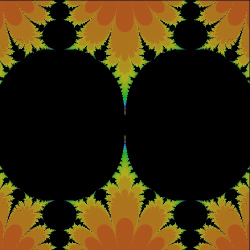 |
k_sine_R1.25.dwg R = 1.25 case 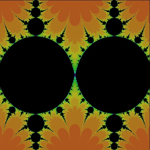 |
k_sine_R1.50.dwg R = 1.50 case 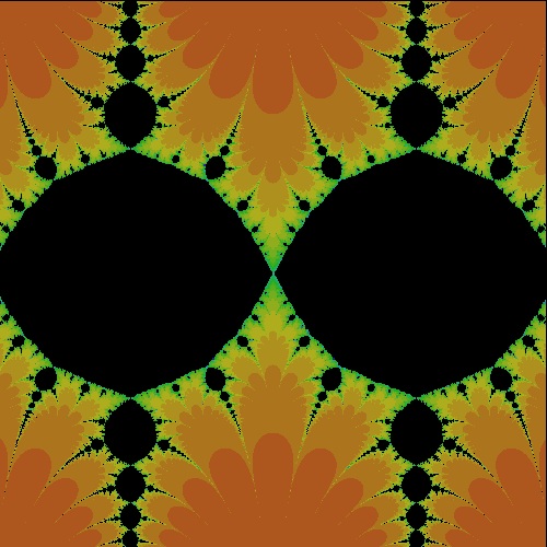 |
k_sine_R2.00.dwg R = 2.00 case 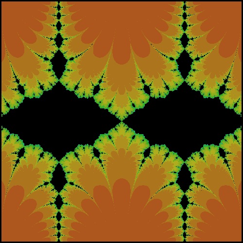 |
k_sine_R2.50.dwg R = 2.50 case 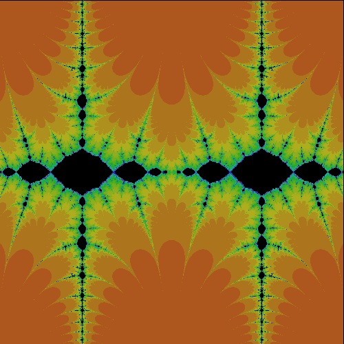 |
(2) Pure Imaginary cases
Data range : (-3.0 -3.0) - (3.0 3.0)
Max Iteration: 50
Click a mouse on the picture for a larger image.
|
k_sine_I0.95.dwg I = 0.95 case 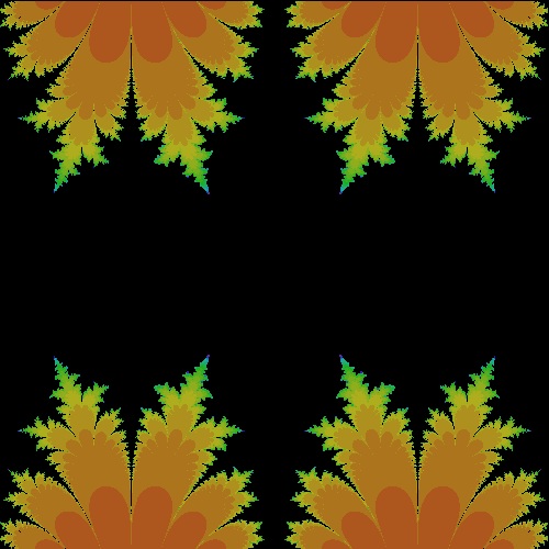 |
k_sine_I1.0.dwg I = 1.0 case 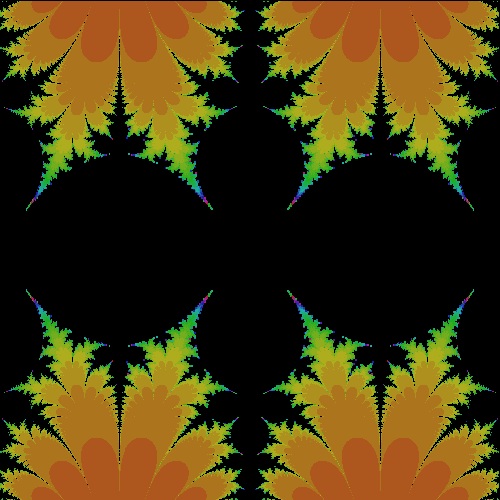 |
k_sine_I1.05.dwg I = 1.05 case 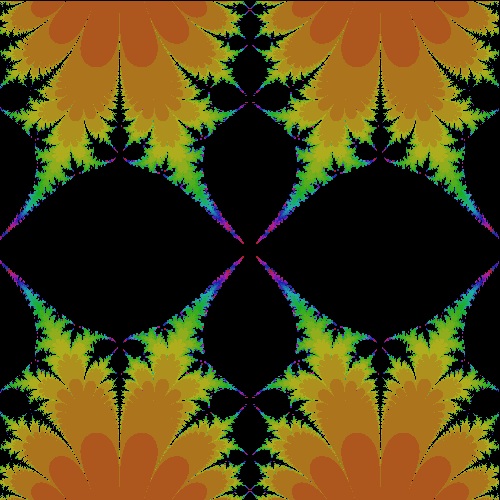 |
k_sine_I1.1.dwg I = 1.1 case 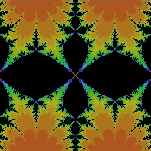 |
k_sine_I1.2.dwg I = 1.2 case 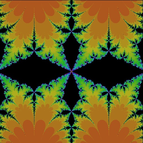 |
|
k_sine_I1.275.dwg I = 1.275 case 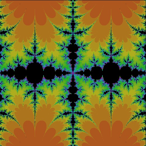 |
k_sine_I1.35.dwg I = 1.35 case 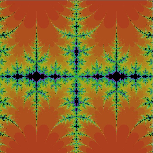 |
k_sine_I1.4.dwg I = 1.4 case 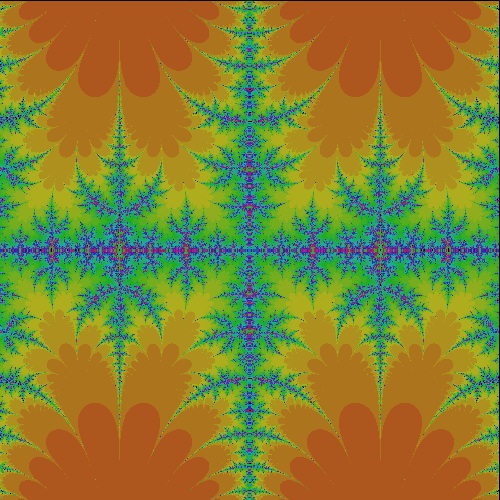 |
k_sine_I2.0.dwg I = 2.0 case 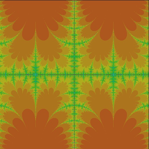 |
k_sine_I3.0.dwg I = 3.0 case 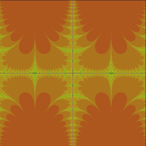 |
(3) k = 1 + i c case, where c = 0 - 2.0
Data range : (-1.5 -1.5) - (1.5 1.5)
Max Iteration: 50
Click a mouse on the picture for a larger image.
|
k_sine_0.00000.dwg I = 0.00 case 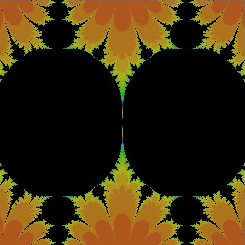 |
k_sine_0.01048.dwg I = 0.01048 case 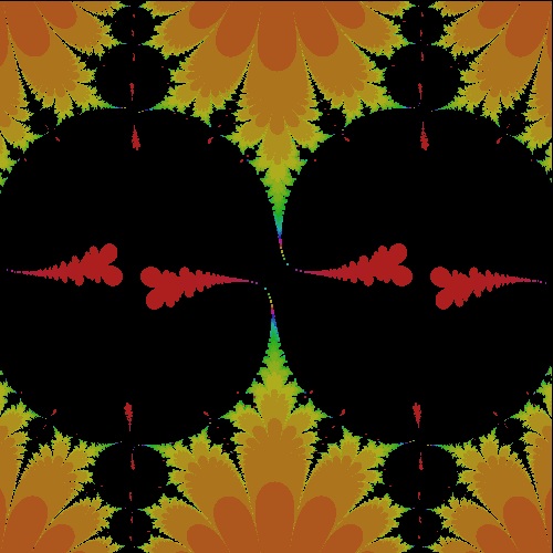 |
k_sine_0.01060.dwg I = 0.01060 case 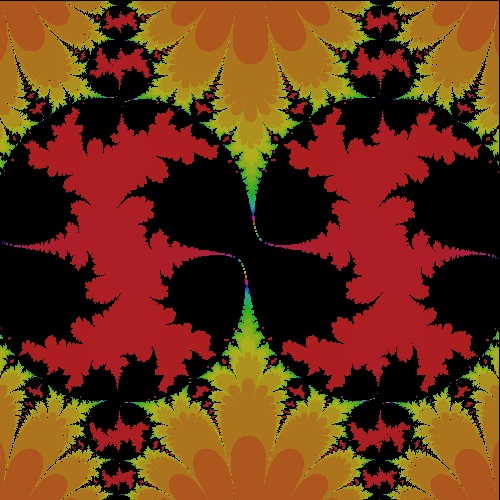 |
k_sine_0.01080.dwg I = 0.01080 case 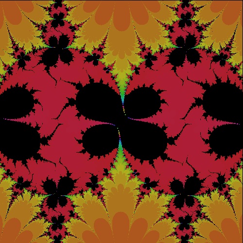 |
k_sine_0.01500.dwg I = 0.01500 case 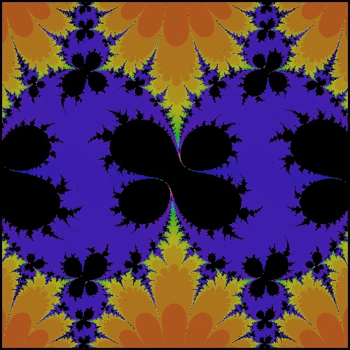 |
|
k_sine_0.02500.dwg I = 0.02500 case 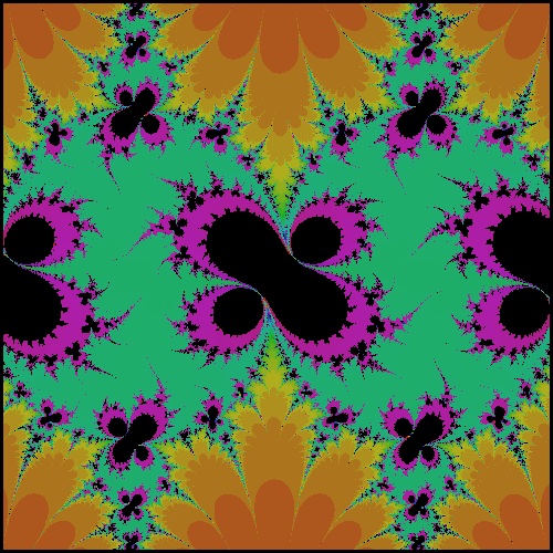 |
k_sine_0.05000.dwg I = 0.05000 case 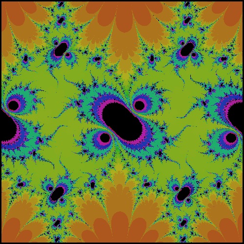 |
k_sine_0.10000.dwg I = 0.10000 case 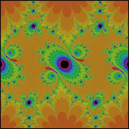 |
k_sine_0.20000.dwg I = 0.20000 case 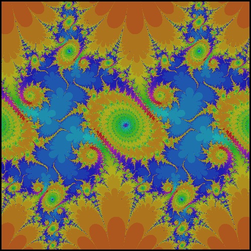 |
k_sine_0.30000.dwg I = 0.30000 case 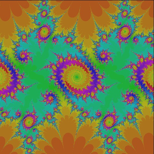 |
|
k_sine_0.40000.dwg I = 0.40000 case 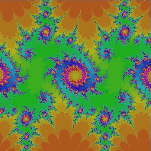 |
k_sine_0.50000.dwg I = 0.50000 case 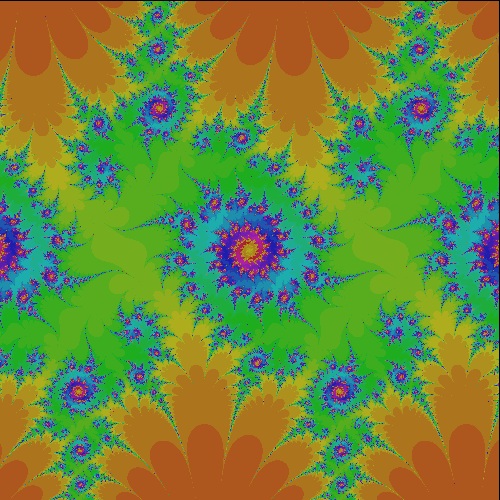 |
k_sine_0.70000.dwg I = 0.70000 case 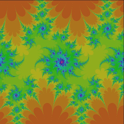 |
k_sine_1.00000.dwg I = 1.00000 case 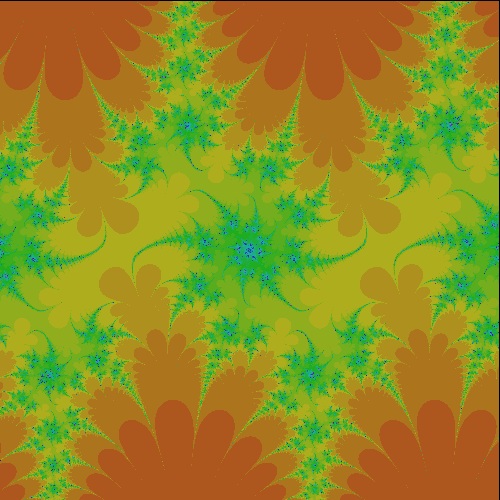 |
k_sine_1.90000.dwg I = 1.90000 case 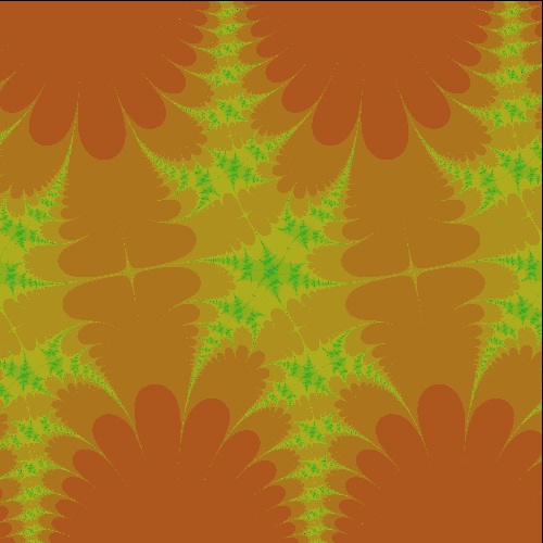 |
Zoom up of some selected cases
Data range : (-1.5 -1.5) - (1.5 1.5)
Max Iteration: 300
Click a mouse on the picture for a larger image.
|
k_sine_1.0_0.05.dwg k = 1, 0.05 case 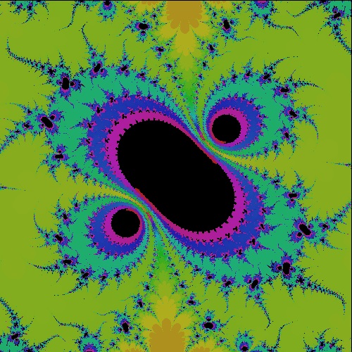 |
k_sine_1.0_0.10.dwg k = 1, 0.10 case 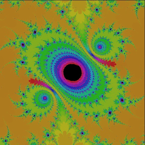 |
k_sine_1.0_0.20.dwg k = 1, 0.20 case 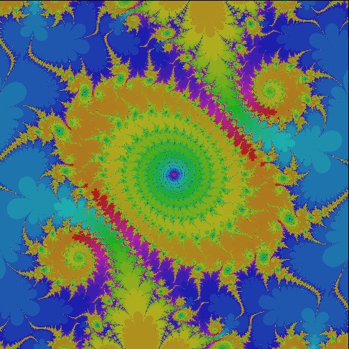 |
k_sine_1.0_0.30.dwg k = 1, 0.30 case 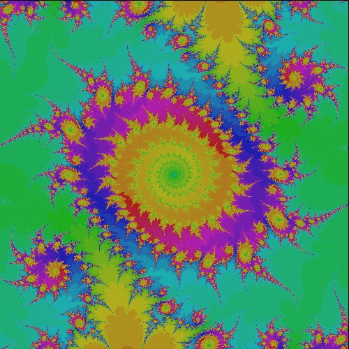 |
k_sine_1.0_0.40.dwg k = 1, 0.40 case 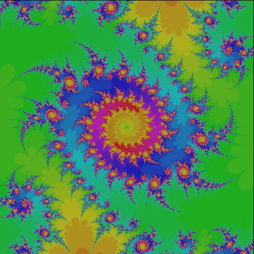 |
(4) General case k = a + ib (a = 0.6 - 0.7; b = 0.8 - 0.9)
Click a mouse on the picture for a larger image.
Data range : (-1.5 -1.5) - (1.5 1.5)
Max Iteration: 300
|
k_sine_0.600_0.800_3x3 k = 0.6, 0.8 case 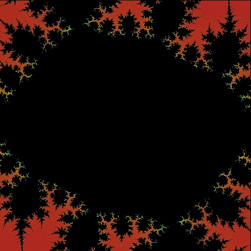 |
k_sine_0.6005_0.8005_3x3 k = 0.6005, 0.8005 case 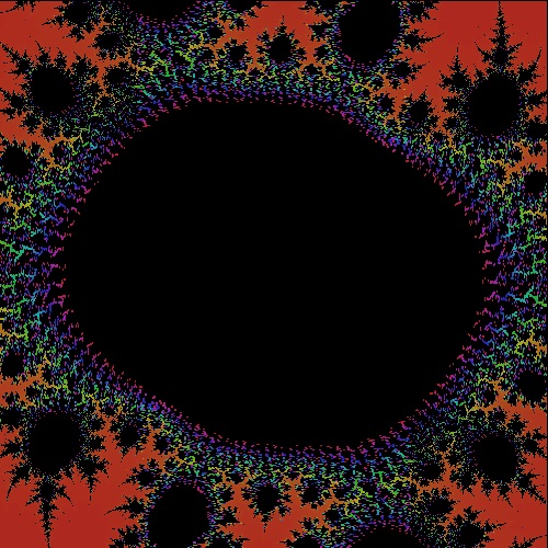 |
k_sine_0.601_0.801_3x3 k = 0.601, 0.801 case 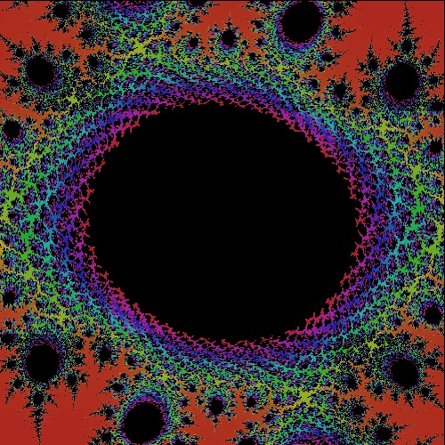 |
k_sine_0.602_0.802_3x3 k = 0.602, 0.802 case 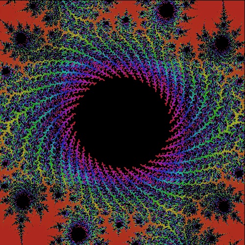 |
k_sine_0.605_0.805_3x3 k = 0.605, 0.805 case 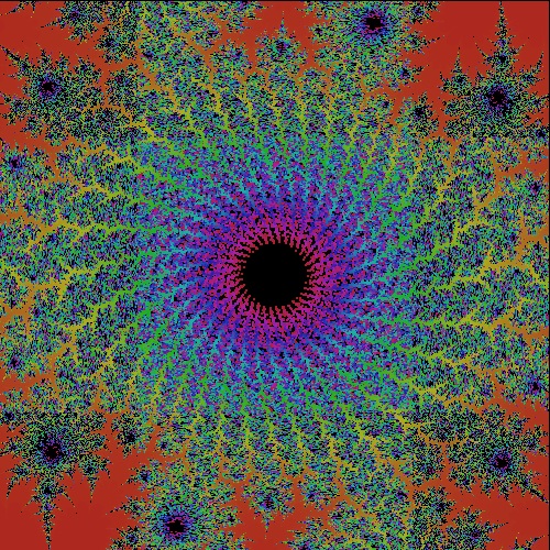 |
|
k_sine_0.608_0.808_3x3 k = 0.608, 0.808 case 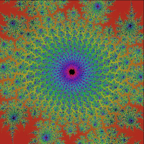 |
k_sine_0.610_0.810_3x3 k = 0.610, 0.810 case 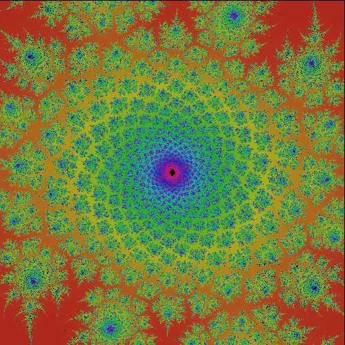 |
k_sine_0.615_0.815_3x3 k = 0.615, 0.815 case 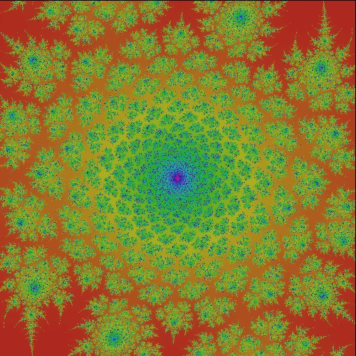 |
k_sine_0.620_0.820_3x3 k = 0.620, 0.820 case 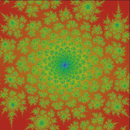 |
k_sine_0.630_0.830_3x3 k = 0.630, 0.830 case 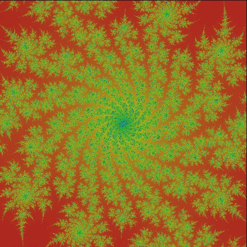 |
(5) Zoom up of 0.61 + i 0.81 case
Click a mouse on the picture for a larger image.
Max Iteration: 300
|
k_sine_0.610_0.810_z1 1.5 x 1.5 frame 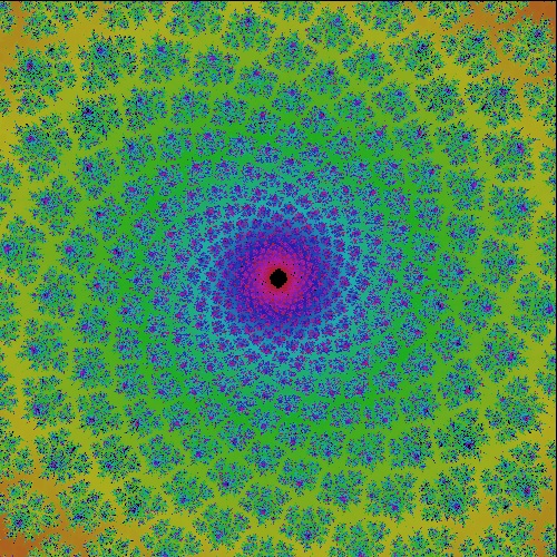 |
k_sine_0.610_0.810_z2 1.0 x 1.0 frame 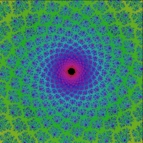 |
k_sine_0.610_0.810_z3 0.5 x 0.5 frame 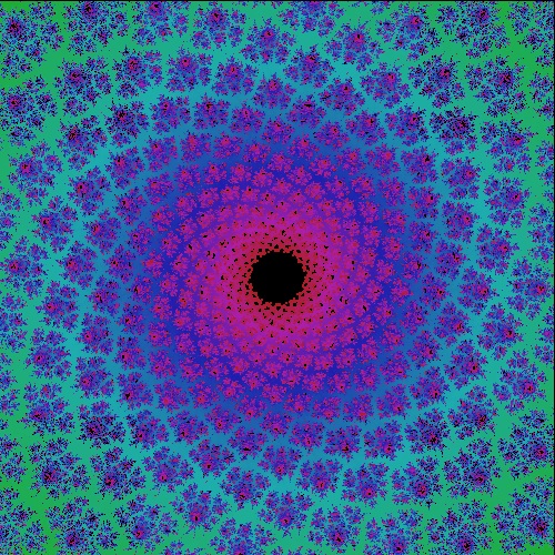 |
k_sine_0.610_0.810_z4 0.2 x 0.2 frame 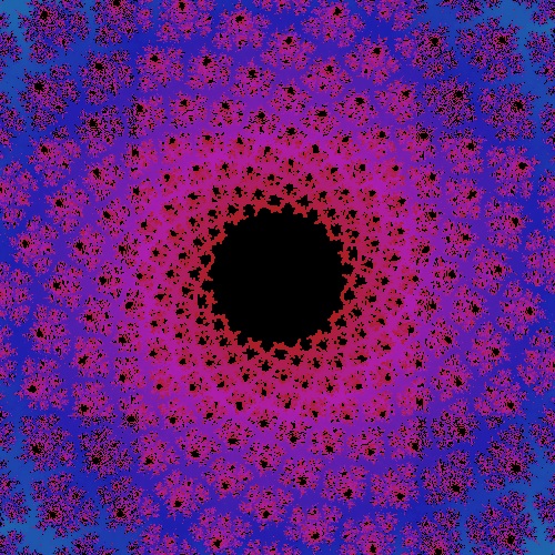 |
k_sine_0.610_0.810_z5 0.1 x 0.1 frame 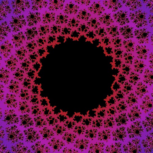 |
5.2.3 Complex Cosine function
How to create the following colored drawings :In addition to loading my_tools.lsp, fractal_tools.lsp must be loaded for all the following execution.
Load fractal_tools.lsp (load "fractal_tools")
Load julia_general.lsp (load "julia_general")
Then from command line, type julia_kcosine
(1) Pure Imaginary cases
Click a mouse on the picture for a larger image.
Data range : (-3.0 -3.0) - (3.0 3.0)
Max Iteration: 50
|
k_cos_I0.6650_50.dwg I = 0.6650 case 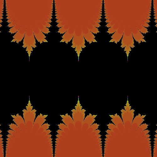 |
k_cos_I0.6663_50.dwg I = 0.6663 case 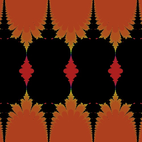 |
k_cos_I0.6664_50.dwg I = 0.6664 case 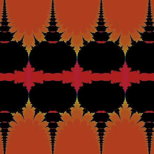 |
k_cos_I0.6666_50.dwg I = 0.6666 case 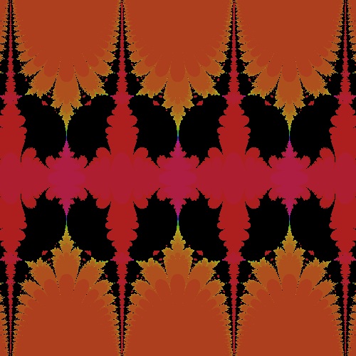 |
k_cos_I0.6670_50.dwg I = 0.6670 case 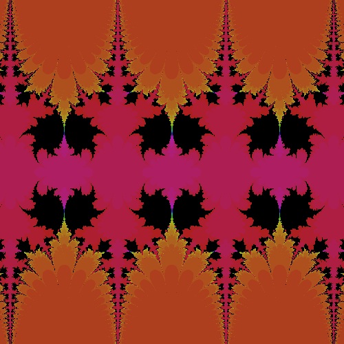 |
|
k_cos_I0.6700_50.dwg I = 0.6700 case 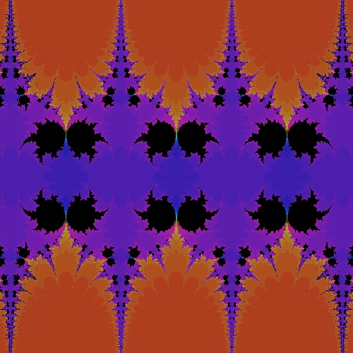 |
k_cos_I0.6800_50.dwg I = 0.6800 case 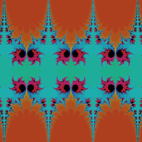 |
k_cos_I0.7000_50.dwg I = 0.7000 case 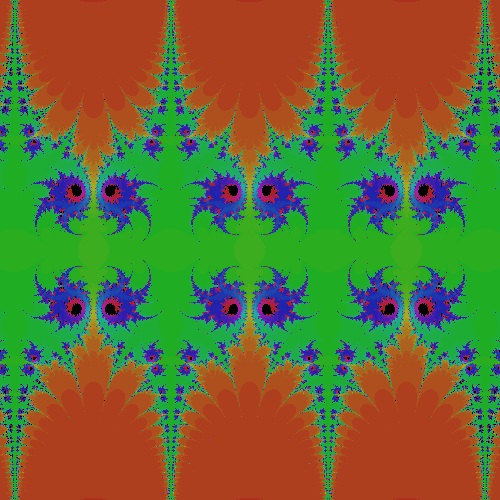 |
k_cos_I0.7500_50.dwg I = 0.7500 case 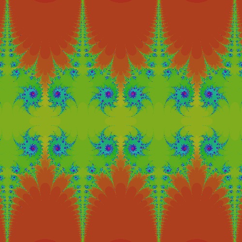 |
k_cos_I1.0000_50.dwg I = 1.0000 case 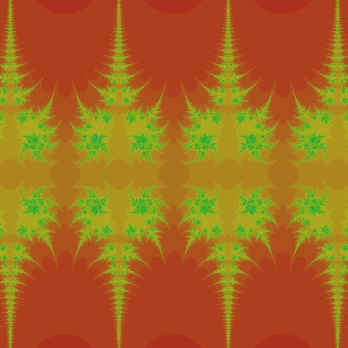 |
(2) Pure Real cases
Click a mouse on the picture for a larger image.
Data range : (-1.5 -1.5) - (1.5 1.5)
Max Iteration: 50
|
k_cos_R3.1000_50 R = 3.1000 case 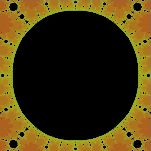 |
k_cos_R2.9700_50 R = 2.9700 case 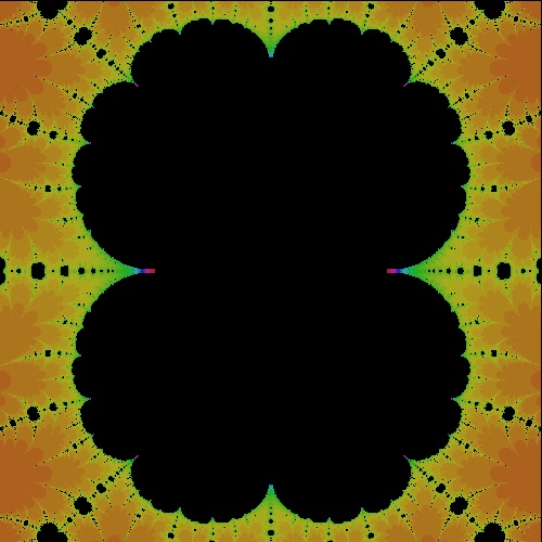 |
k_cos_R2.9690_50g R = 2.9690 case 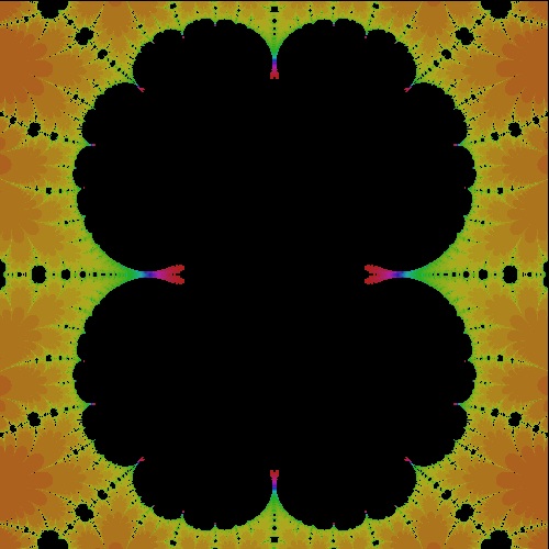 |
k_cos_R2.9680_50 R = 2.9680 case 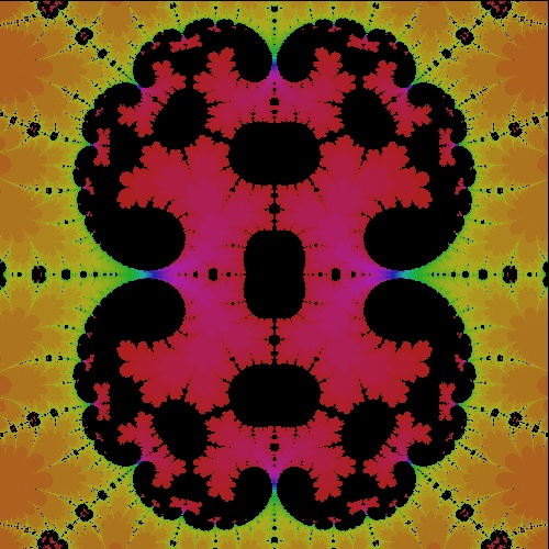 |
k_cos_R2.9670_50 R = 2.9670 case 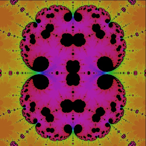 |
|
k_cos_R2.9660_50 R = 2.9660 case 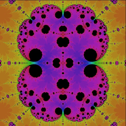 |
k_cos_R2.9650_50 R = 2.9650 case 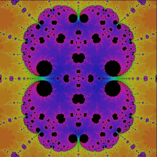 |
k_cos_R2.9600_50g R = 2.9600 case 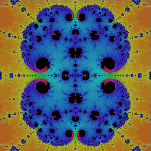 |
k_cos_R2.9500_50 R = 2.9500 case 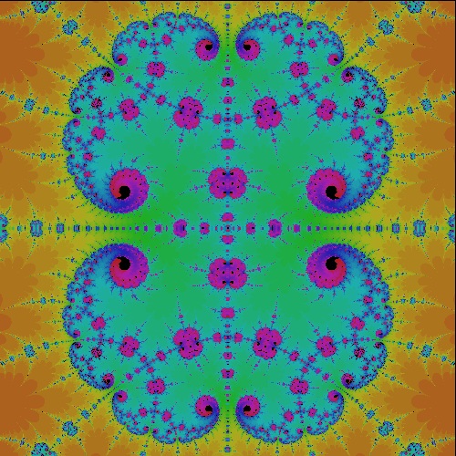 |
k_cos_R2.9400_50 R = 2.9400 case 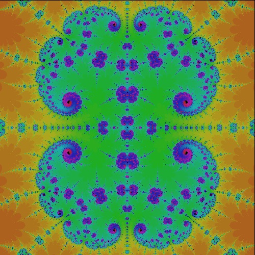 |
|
k_cos_R2.9300_50 R = 2.9300 case 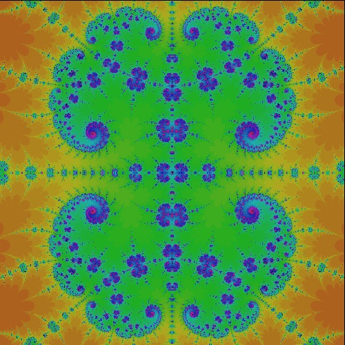 |
k_cos_R2.9200_50 R = 2.9200 case 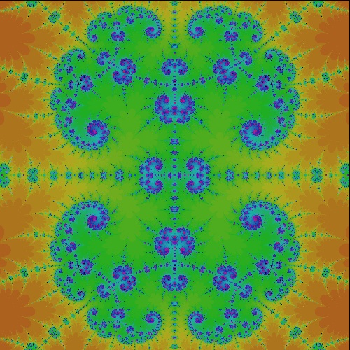 |
k_cos_R2.9100_50g R = 2.9100 case 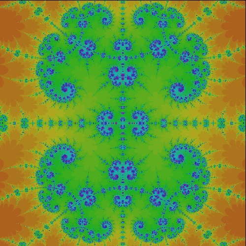 |
k_cos_R2.9000_50 R = 2.9000 case 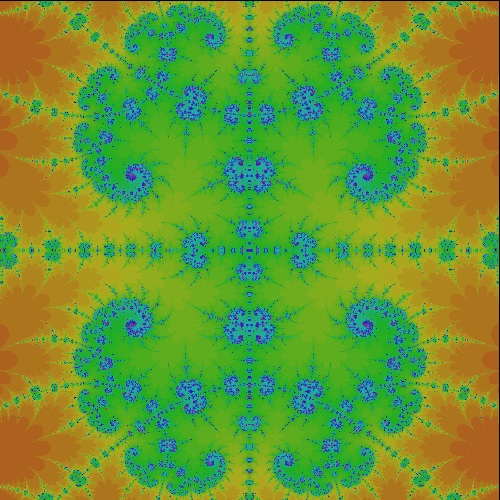 |
k_cos_R2.8000_50 R = 2.8000 case 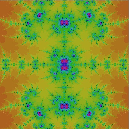 |
|
k_cos_R2.5000_50 R = 2.5000 case 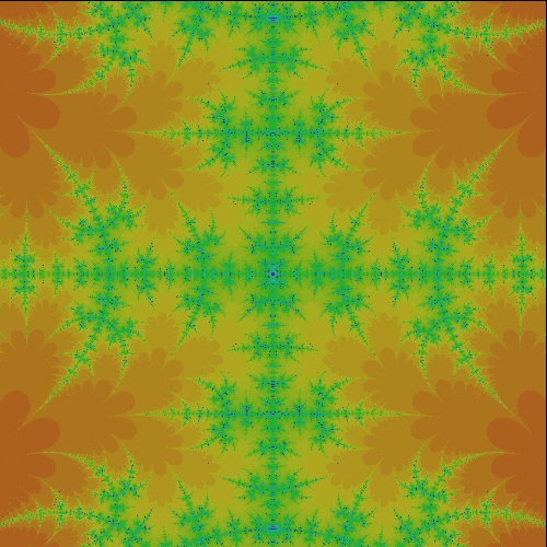 |
k_cos_R2.0000_50 R = 2.0000 case 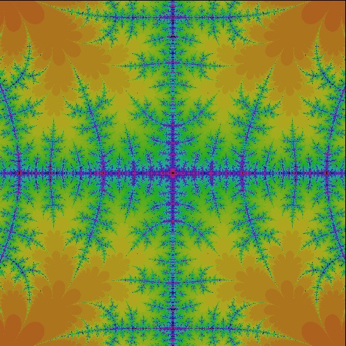 |
k_cos_R1.9500_50g R = 1.9500 case 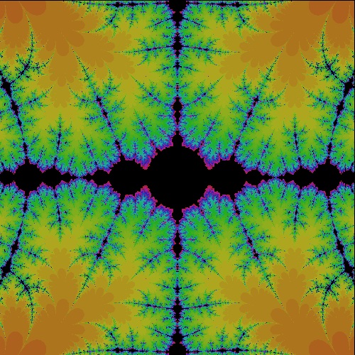 |
k_cos_R1.9000_50 R = 1.9000 case 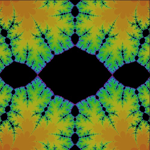 |
k_cos_R1.8000_50 R = 1.8000 case 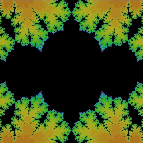 |
(3) Zoom up of selected cases
Click a mouse on the picture for a larger image.
Max Iteration: 50
|
k_cos_I0.68_50_z k = i 0.68 case 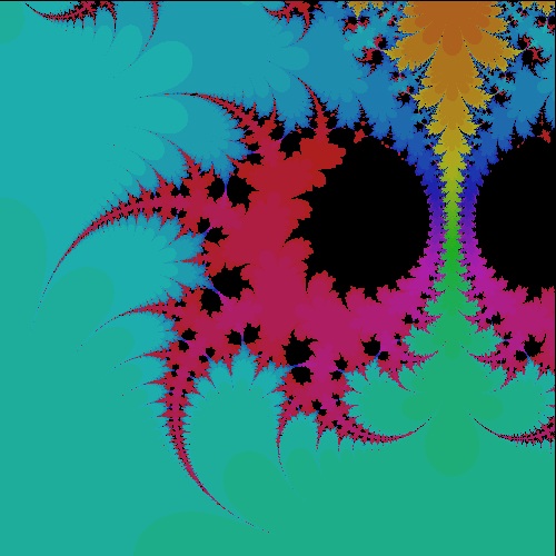 |
k_cos_I0.70_50_z k = i 0.70 case 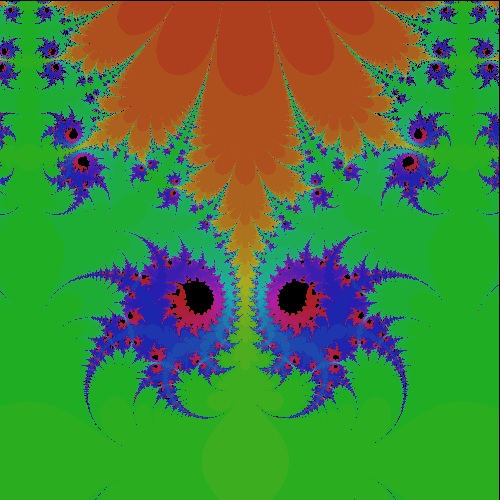 |
k_cos_R2.80_50_z k = 2.80 + i 0 case 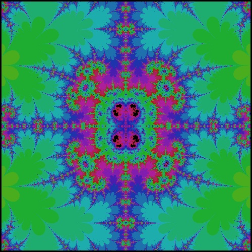 |
k_cos_R2.94_50_z k = 2.94 + i 0 case 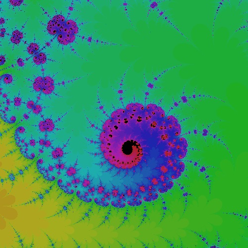 |
k_cos_R2.95_50_z k = 2.95 + i 0 case 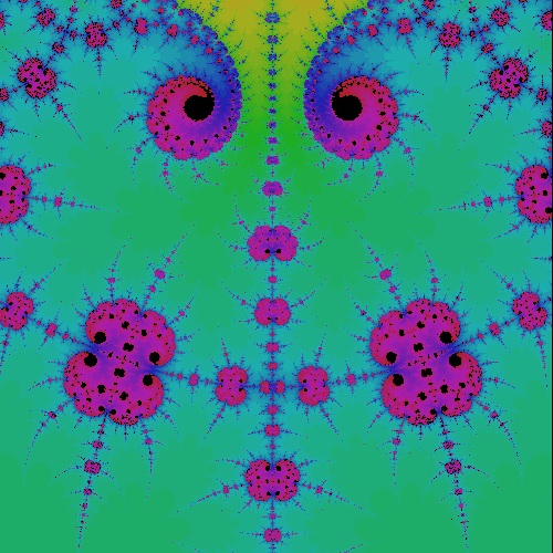 |
(4) General case k = a + ib (a = 2.90 - 3.10; b = 0.15 - 0.40)
Click a mouse on the picture for a larger image.
Data range : (-1.5 -1.5) - (1.5 1.5)
Max Iteration: 300
(4.1) a = 2.90 ; b= 0.187 - 0.250 case
|
k_cos_2.90_0.187_300 k = 2.9, 0.187 case 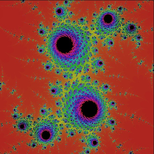 |
k_cos_2.90_0.188_300 k = 2.9, 0.188 case 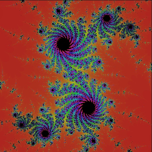 |
k_cos_2.90_0.190_300 k = 2.9, 0.190 case 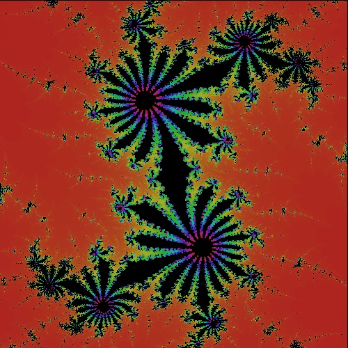 |
k_cos_2.90_0.191_300 k = 2.9, 0.191 case 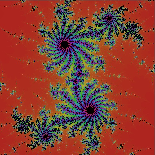 |
k_cos_2.90_0.195_300 k = 2.9, 0.195 case 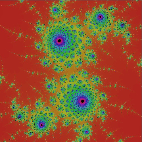 |
|
k_cos_2.90_0.200_300 k = 2.9, 0.200 case 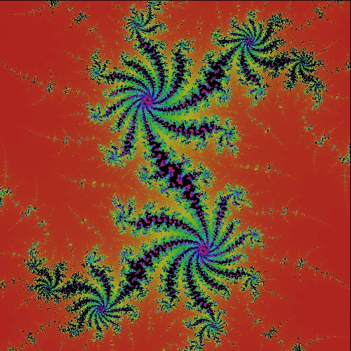 |
k_cos_2.90_0.230_300 k = 2.9, 0.230 case 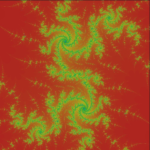 |
k_cos_2.90_0.237_300 k = 2.9, 0.237 case 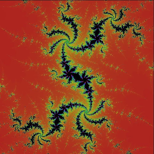 |
k_cos_2.90_0.240_300 k = 2.9, 0.240 case 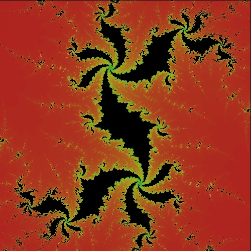 |
k_cos_2.90_0.250_300 k = 2.9, 0.250 case 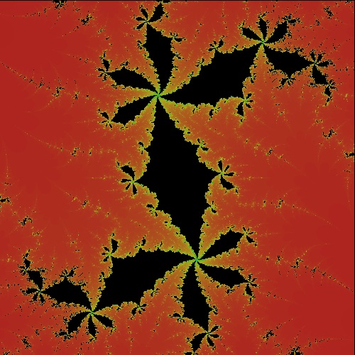 |
(4.2) a = 2.95 ; b= 0.281 - 0.298 case
|
k_cos_2.95_0.281_300 k = 2.95, 0.281 case 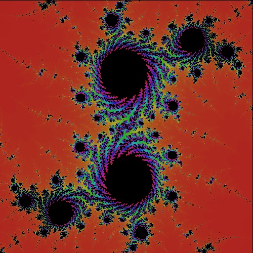 |
k_cos_2.95_0.285_300 k = 2.95, 0.285 case 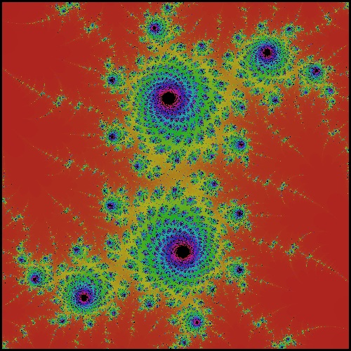 |
k_cos_2.95_0.289_300 k = 2.95, 0.289 case 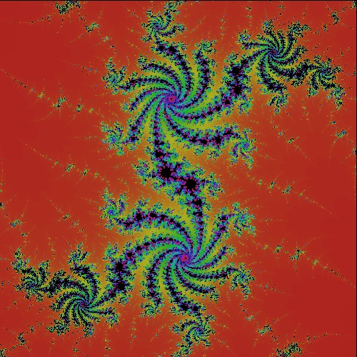 |
k_cos_2.95_0.297_300 k = 2.95, 0.297 case 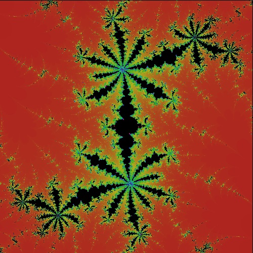 |
k_cos_2.95_0.298_300 k = 2.95, 0.298 case 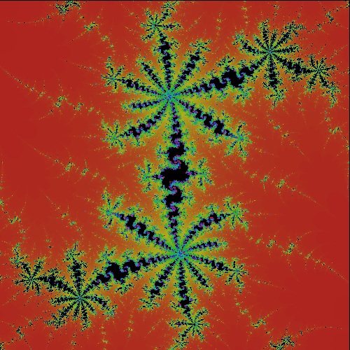 |
(4.3) a = 3.00 ; b= 0.330 - 0.400 case
|
k_cos_3.00_0.330_300 k = 3.00, 0.330 case 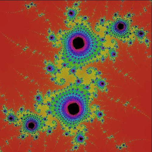 |
k_cos_3.00_0.333_300 k = 3.00, 0.333 case 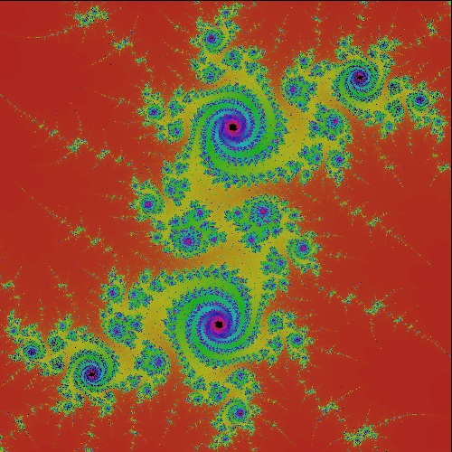 |
k_cos_3.00_0.334_300 k = 3.00, 0.334 case 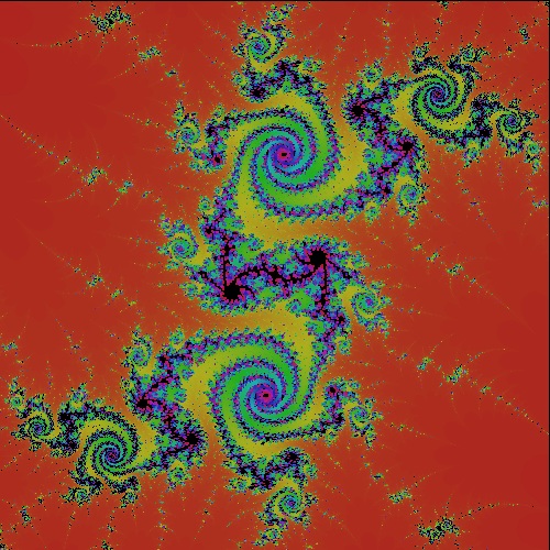 |
k_cos_3.00_0.335_300 k = 3.00, 0.335 case 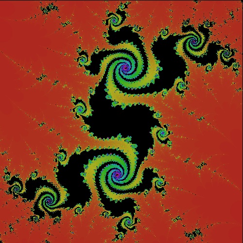 |
k_cos_3.00_0.337_300 k = 3.00, 0.337 case 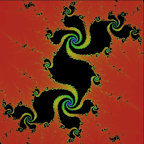 |
|
k_cos_3.00_0.340_300 k = 3.00, 0.340 case 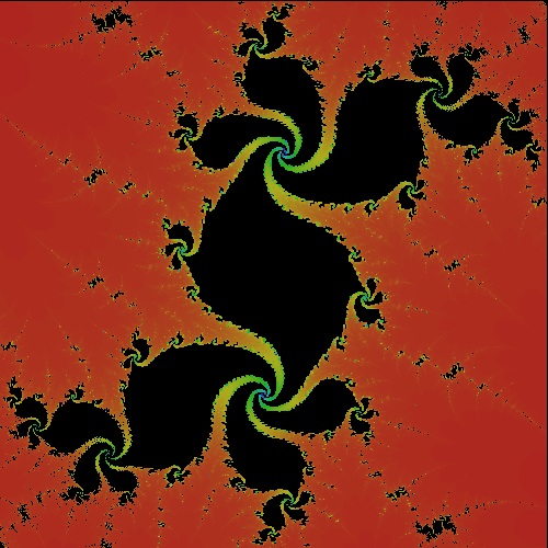 |
k_cos_3.00_0.350_300 k = 3.00, 0.350 case 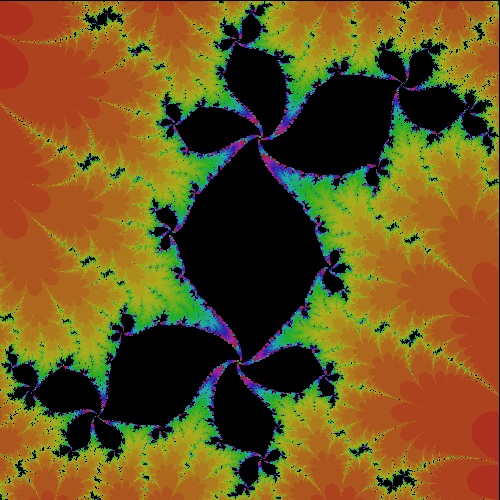 |
k_cos_3.00_0.370_300 k = 3.00, 0.370 case 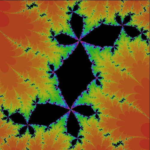 |
k_cos_3.00_0.390_300 k = 3.00, 0.390 case 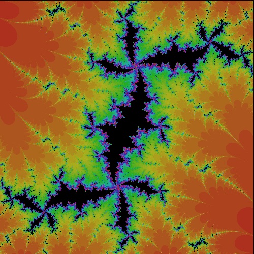 |
k_cos_3.00_0.400_300 k = 3.00, 0.400 case 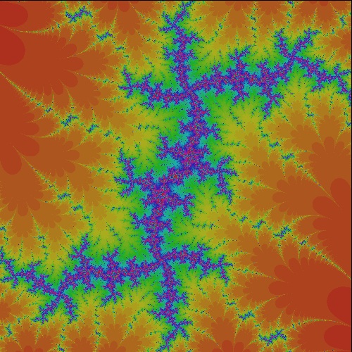 |
(4.3) a = 3.10 ; b= 0.378 - 0.395 case
|
k_cos_3.10_0.378_300 k = 3.10, 0.378 case 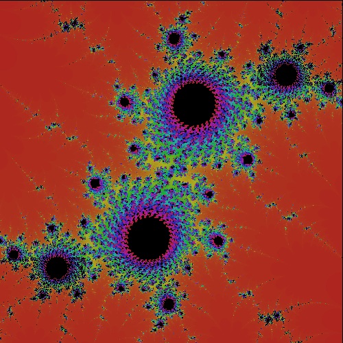 |
k_cos_3.10_0.380_300 k = 3.10, 0.380 case 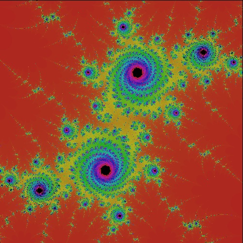 |
k_cos_3.10_0.385_300 k = 3.10, 0.385 case 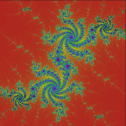 |
k_cos_3.10_0.390_300 k = 3.10, 0.390 case 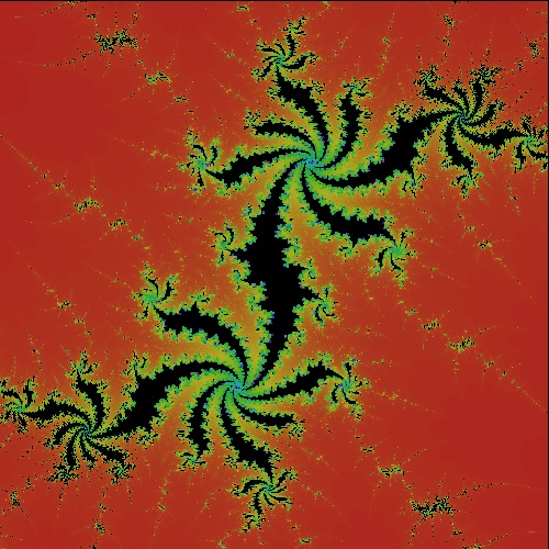 |
k_cos_3.10_0.395_300 k = 3.10, 0.395 case 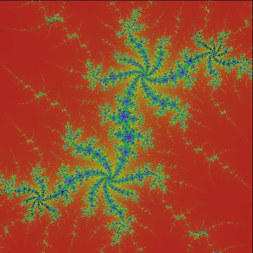 |
5.2.4 Complex Exponential function
How to create the following colored drawings :In addition to loading my_tools.lsp, fractal_tools.lsp must be loaded for all the following execution.
Load fractal_tools.lsp (load "fractal_tools")
Load julia_general.lsp (load "julia_general")
Then from command line, type julia_kexp
(1) Pure imaginary case ; pi and 2 pi cases
|
exp_0.00_3.14_50 k = 3.14 case 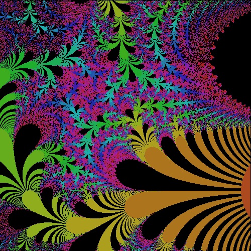 |
k_exp_0.00_6.28_50 k = 6.28 case 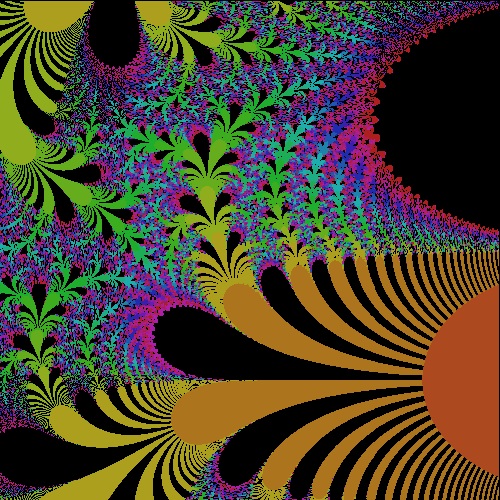 |
k_cos_3.10_0.385_300 k = 3.10, 0.385 case |
k_cos_3.10_0.390_300 k = 3.10, 0.390 case |
k_cos_3.10_0.395_300 k = 3.10, 0.395 case |
(2) Pure real case ; 0.20 - 1.0 cases
|
exp_0.2000_0.0_50 k = 0.20 case  |
k_exp_0.3670_0.0_50 k = 0.367 case 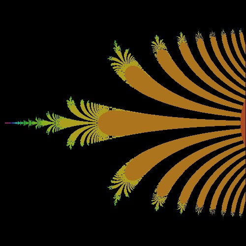 |
k_exp_0.3700_0.0_50 k = 0.370 case 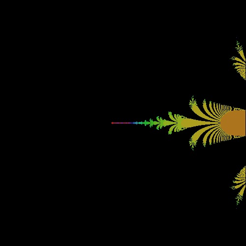 |
k_exp_0.3708_0.0_50 k = 0.3708 case 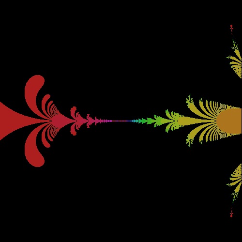 |
k_exp_0.3710_0.0_50 k = 0.3710 case 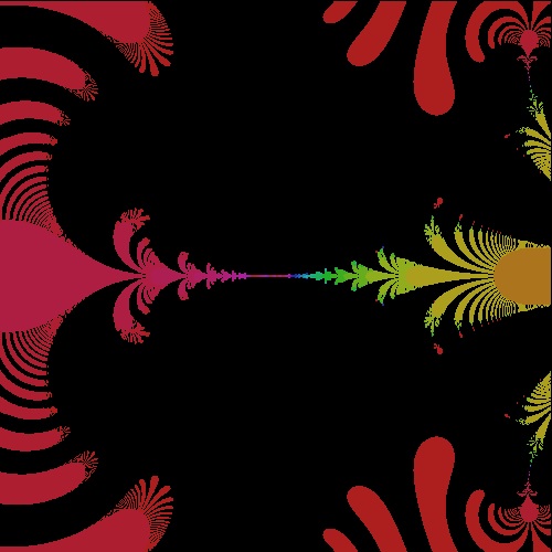 |
|
exp_0.3750_0.0_50 k = 0.375 case 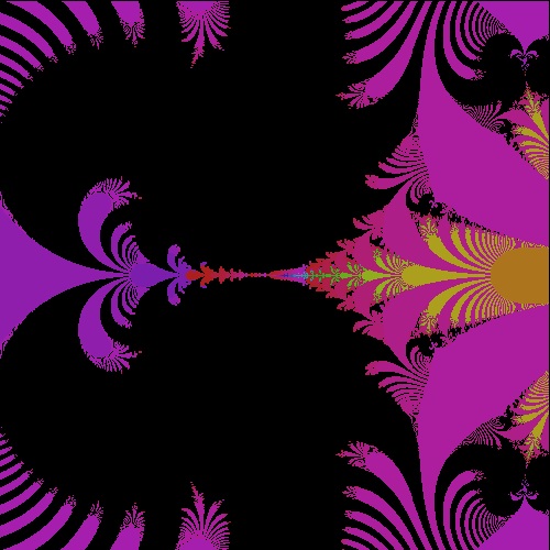 |
k_exp_0.3800_0.0_50 k = 0.380 case 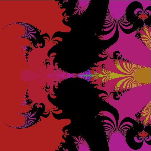 |
k_exp_0.3850_0.0_50 k = 0.385 case 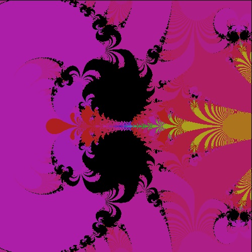 |
k_exp_0.3900_0.0_50 k = 0.390 case 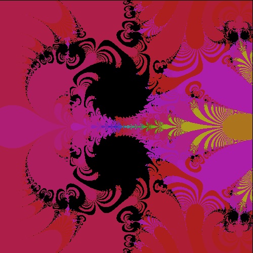 |
k_exp_0.4000_0.0_50 k = 0.400, 0.395 case 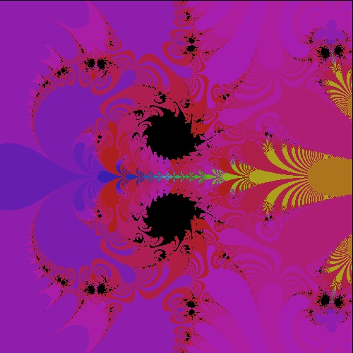 |
|
exp_0.4100_0.0_50 k = 0.41 case 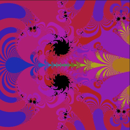 |
k_exp_0.4200_0.0_50 k = 0.42 case 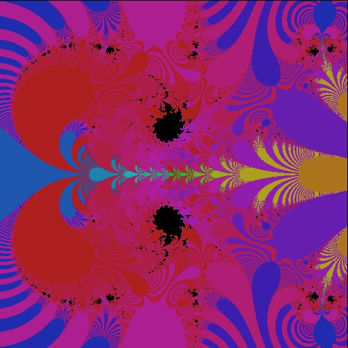 |
k_exp_0.4300_0.0_50 k = 0.43, 0.385 case 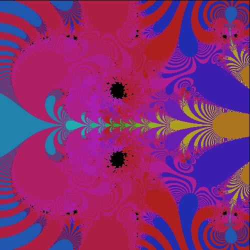 |
k_exp_0.4400_0.0_50 k = 0.44, 0.390 case 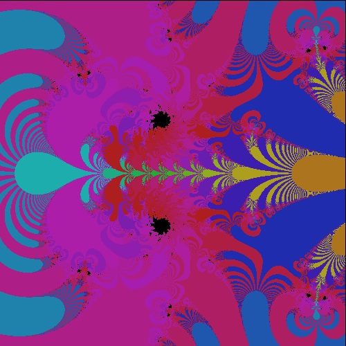 |
k_exp_0.4500_0.0_50 k = 0.45, 0.395 case 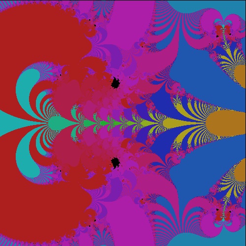 |
|
exp_0.5000_0.0_50 k = 0.5 case 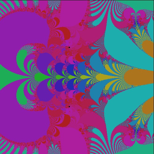 |
k_exp_0.6000_0.0_50 k = 0.6 case 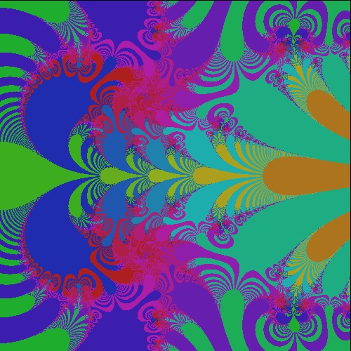 |
k_exp_0.7000_0.0_50 k = 0.7, 0.385 case 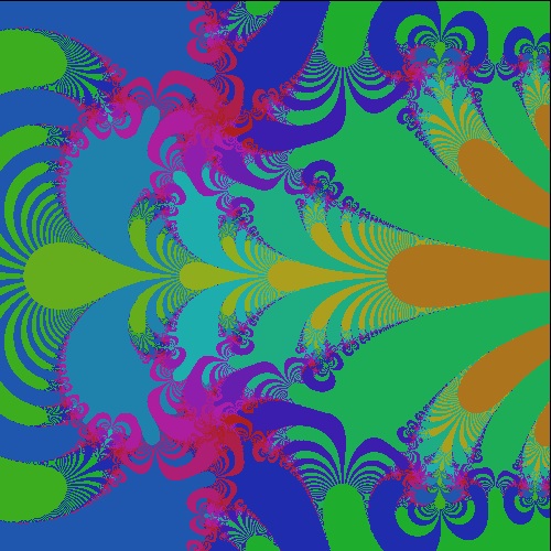 |
k_exp_0.8000_0.0_50 k = 0.8, 0.390 case 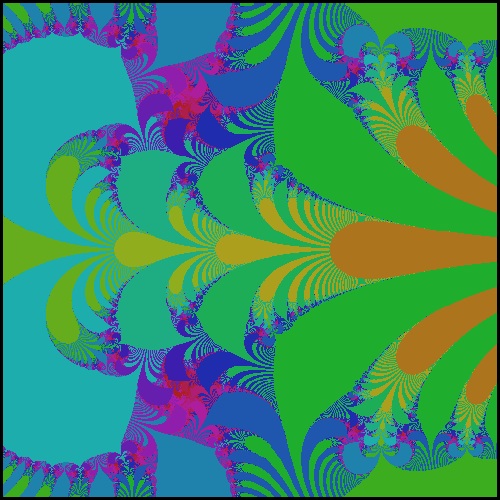 |
k_exp_1.0000_0.0_50 k = 1.0, 0.395 case 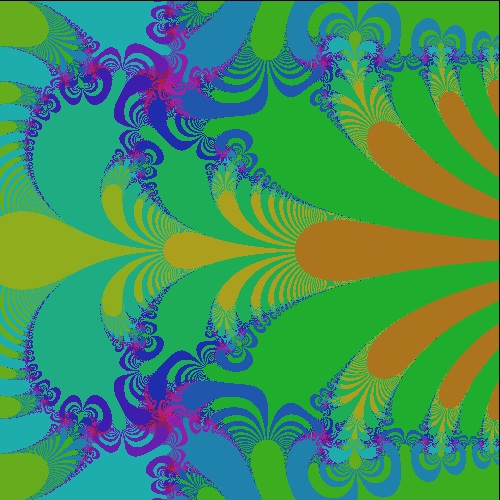 |
(3) General complex cases
|
exp_1.00_0.20_50 k = 1.00, 0.20 case 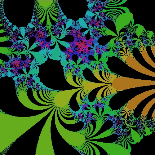 |
k_exp_1.0_2.0_50 k = 1.0, 2.0 case 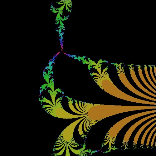 |
k_exp_M2.5_1.50_50 k = -2.5, 1.50 case 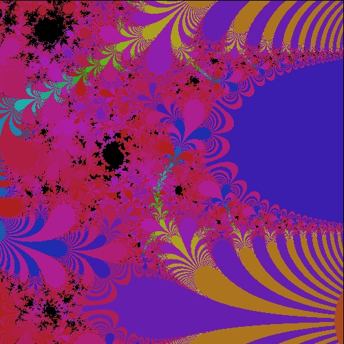 |
k_exp_M2.7_1.50_50 k = -2.7, 1.50 case  |
k_exp_m4.0_1.0_50 k = -4.0, 1.0 case 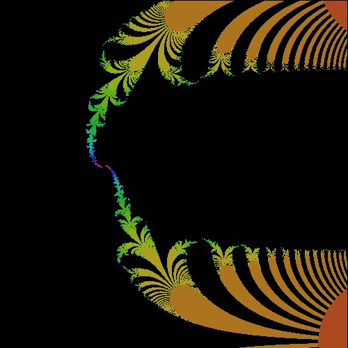 |
5.2.5 Hyperbolic sine function
5.2.6 Hyperbolic cosine function
5.2.1 Other and higher degree polynomial functions
Conjugate function case: If the sign of the imaginary part is changed from positive to negative ,i.e. z = x - i y, it is called "conjugate".6. Mandelbrot Set
6.1 Mandelbrot Set
6.2 Mandelbrot-like Set for other functions
7. IFS(Iterated Funtion System)
References
There are many books written on this topics. The books referenced in posting the above contents
are listed in four groups:
1. Classic books
2. Introduction to the concept
3. Generally for writing computer codes
4. College Math-textbook type
5. General reference
1. Classic books
- Mandelbrot, Benoit B.: The Fractal Geometry of Nature. Freeman, 1977.
- Peitgen, Heinz-Otto., Richter, Peter H.: The Beauty of Fractals - Images of Complex Dynamical Systems . Springer-Verlag, 1986.
- Przemyslaw Prusinkiewicz, Aristid Lindenmayer: The Algorithmic Beauty of Plants. Springer-Verlag, 1990.
- Peitgen Heinz-Otto., Jurgens,H.,Saupe,D.: Chaos and Fractals - New Frontiers of Science. Springer-Verlag, 1992.
- Barnsley,Michael F.: Fractals Everywhere. Academic Press. 1993.
- Flake, Gary W.: The Computational Beauty of Nature - Computer Explorations of Fractals,Chaos, Complex Systems, and Adaptaions. MIT Press. 1998.
- Mumford,D.,Series C.,Wright,D.: Indra's Pearls - The Vision of Felix Klein. Cambridge Univ. Press. 2002.
2. Introduction to the concept
- Lauwerier, Hans A.: Fractal - Endlessly Repeated Geometrical Figures. Princeton Univ. Press. 1991.
- McGuire, Michael D.: An Eye for Fractals. Addison-Wesley. 1991.
- Briggs, John: Fractal - The Patterns of Chaos. Simon and Schuster, 1992.
- Nigel Lesmoir-Gordon, Will Rood, Ralph Edney: Introductions - Fractal Geometry. Totem Books, 2000.
- Clark, Arthur,C.,et al: The Colours of Infinity - The Beauty and Power of Fractals. Clear Books, 2006.
- Smith,Leonard A.: Chaos - A Very Short Introduction. Oxford Univ. Press, 2007.
- Peitgen Heinz-Otto., Saupe,Dietmar.,Editors: The Science of Fractal Images. Springer-Verlag, 1988.
- Laplante, Phil.: Fractal Mania. Windcress/McGraw-Hill,1994..
- Stevens,Robert T.: Creating Fractals. Charles River Media, 2005.
- Ahlfors,Lars V.: Complex Analysis - An Introduction to the Theory of Analytic Functions of One Complex Variable. MaGraw-Hill. 1953.
- Devaney,Robert L.: Chaos, Fractals and Dynamics-Computer Experiments in Mathematics. Addison-Wesley,1990.
- Devaney,Robert L.: A First Course in Chaotic Dynamical Systems- Theory and Experiment. Addison-Wesley,1992.
- Sagan,Hans.: Space-Filling Curves. Springer-Verlag. 1994.
- Devaney,Robert L.: The Mandelbrot and Julia Sets - A Tool Kit of Dynamic Activities. Key Curriculum Press. 2000.
- Walser,Hans.: The Golden Section. Mathematical Association of America, 2001.
- Devaney,Robert L.: An Introduction to Chaotic Dynamical Systems. WestView Press. 2003.
- Davies,Brian: Exploring Chaos - theory and experiment. WestView,2004.
- Falconer,Kenneth J.: Fractal Geometry - Mathematical Foundations and Applications. John Wiley and Sons. 1990.
- Falconer,Kenneth J.: Techniques in Fractal Geometry. John Wiley and Sons. 1997.
- Lorenz,Edward N.: The Essence of Chaos. Univ of Washington Press. 1993.
- Mandelbrot, Benoit B.: Fractal and Chaos - The Mndelbrot Set and Beyond. Springer-Verlag. 2004.
- Barnsley, Michael F.: SuperFractals - Pattern of Nature. Cambridge Univ. Press. 2006.